Highly Charged Ion (HCI) Lines from NIST ASD

Motivation

We often find ourselves hard coding line center positions into mass, which is prone to errors and can be tedious when there are many lines of interest to insert. In addition, the line positions would need to be manually updated for any changes in established results. In the case of highly charged ions, such as those produced in an electron beam ion trap (EBIT), there is a vast number of potential lines coming from almost any charge state of almost any element. Luckily, these lines are well documented through the NIST Atomic Spectral Database (ASD). Here, we have parsed a NIST ASD SQL dump and converted it into an easily Python readable pickle file. The hci_lines.py module implements the NIST_ASD class, which loads that pickle file and contains useful functions for working with the ASD data. It also automatically adds in some of the more common HCI lines that we commonly use in our EBIT data analyses.

Exploring the methods of class NIST_ASD

The class NIST_ASD can be initialized without arguments if the user wants to use the default ASD pickle file. This file is located at mass/calibration/nist_asd.pickle. A custom pickle file can be used by passing in the pickleFilename argument during initialization. The methods of the NIST_ASD class are described below:

class mass.calibration.hci_lines.NIST_ASD(pickleFilename=None)

Class for working with a pickled atomic spectra database

getAvailableElements()

Returns a list of all available elements from the ASD pickle file

getAvailableLevels(element, spectralCharge, requiredConf=None, requiredTerm=None, requiredJVal=None, maxLevels=None, units='eV', getUncertainty=True)

For a given element and spectral charge state, return a dict of all known levels from the ASD pickle file

Args:

element: str representing atomic symbol of element, e.g. ‘Ne’ spectralCharge: int representing spectral charge state, e.g. 1 for neutral atoms, 10 for H-like Ne requiredConf: (default None) filters results to those with conf == requiredConf requiredTerm: (default None) filters results to those with term == requiredTerm requiredJVal: (default None) filters results to those with JVal == requiredJVal maxLevels: (default None) the maximum number of levels (sorted by energy) to return units: (default ‘eV’) ‘cm-1’ or ‘eV’ for returned line position. If ‘eV’, converts from database ‘cm-1’ values

getAvailableSpectralCharges(element)

For a given element, returns a list of all available charge states from the ASD pickle file

Args:

element: str representing atomic symbol of element, e.g. ‘Ne’

getSingleLevel(element, spectralCharge, conf, term, JVal, units='eV', getUncertainty=True)

Return the level data for a fully defined element, charge state, conf, term, and JVal.

Args:

element: str representing atomic symbol of element, e.g. ‘Ne’ spectralCharge: int representing spectral charge state, e.g. 1 for neutral atoms, 10 for H-like Ne conf: str representing nuclear configuration, e.g. ‘2p’ term: str representing nuclear term, e.g. ‘2P*’ JVal: str representing total angular momentum J, e.g. ‘3/2’ units: (default ‘eV’) ‘cm-1’ or ‘eV’ for returned line position. If ‘eV’, converts from database ‘cm-1’ values getUncertainty: (default True) if True, includes uncertainties in list of levels

Usage examples

Next, we will demonstrate usage of these methods with the example of Ne, a commonly injected gas at the NIST EBIT.

import mass
import mass.calibration.hci_lines
import numpy as numpy
import pylab as plt

test_asd = mass.calibration.hci_lines.NIST_ASD()
availableElements = test_asd.getAvailableElements()
assert 'Ne' in availableElements
availableNeCharges = test_asd.getAvailableSpectralCharges(element='Ne')
assert 10 in availableNeCharges
subsetNe10Levels = test_asd.getAvailableLevels(element='Ne', spectralCharge=10, maxLevels=6, getUncertainty=False)
assert '2p 2P* J=1/2' in list(subsetNe10Levels.keys())
exampleNeLevel = test_asd.getSingleLevel(element='Ne', spectralCharge=10, conf='2p', term='2P*', JVal='1/2', getUncertainty=False)

print(availableElements[:10])
print(availableNeCharges)
for k, v in subsetNe10Levels.items():
  subsetNe10Levels[k] = round(v, 1)
print(subsetNe10Levels)
print(f'{exampleNeLevel:.1f}')

['Sn', 'Cu', 'Zn', 'Ga', 'Ge', 'As', 'Rb', 'Se', 'Cl', 'Br']
[1, 2, 3, 4, 5, 6, 7, 8, 9, 10]
{'1s 2S J=1/2': 0.0, '2p 2P* J=1/2': 1021.5, '2s 2S J=1/2': 1021.5, '2p 2P* J=3/2': 1022.0, '3p 2P* J=1/2': 1210.8, '3s 2S J=1/2': 1210.8}
1021.5

Functions for generating SpectralLine objects from ASD data

The module also contains some functions outside of the NIST_ASD class that are useful for integration with MASS. First, the add_hci_line function which, takes arguments that are relevant in HCI work, including as element, spectr_ch, energies, widths, and ratios. The function calls mass.calibration.fluorescence_lines.addline, generates a line name with the given parameters, and populates the various fields. 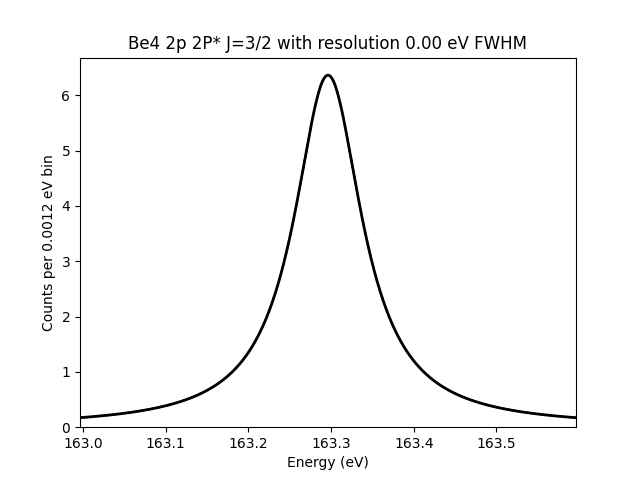As an example, let us create a H-like Be line. Here, we assume a lorentzian width of 0.1 eV.

test_element = 'Be'
test_charge = 4
test_conf = '2p'
test_term = '2P*'
test_JVal = '3/2'
test_level = f'{test_conf} {test_term} J={test_JVal}'
test_energy = test_asd.getSingleLevel(element=test_element, spectralCharge=test_charge,
conf=test_conf, term=test_term, JVal=test_JVal, getUncertainty=False)
test_line = mass.calibration.hci_lines.add_hci_line(element=test_element, spectr_ch=test_charge,
line_identifier=test_level, energies=[test_energy], widths=[0.1], ratios=[1.0])
assert test_line.peak_energy == test_energy

print(mass.spectra[f'{test_element}{test_charge} {test_conf} {test_term} J={test_JVal}'])
print(f'{test_line.peak_energy:.1f}')

SpectralLine: Be4 2p 2P* J=3/2
163.3

The name format for grabbing the line from mass.spectra is shown above. The transition is uniquely specified by the element, charge, configuration, term, and J value. Below, we show what this line looks like assuming a zero-width Gaussian component.

test_line.plot()

The module contains two other functions which are used to easily generate some lines from levels that are commonly observed at the NIST EBIT. These functions are add_H_like_lines_from_asd and add_He_like_lines_from_asd. As the names imply, these functions add H- and He-like lines to mass using the data in the ASD pickle. These functions require the asd and element arguments and also contain the optional maxLevels argument, which works similarly as the argument in the class methods. The module also automatically adds H- and He-like lines for the most commonly used elements, which includes ‘N’, ‘O’, ‘Ne’, and ‘Ar’. Below, we check that common elements are being added as spectralLine objects and then add some of the lower order H- and He-like Ga lines.

print([mass.spectra['Ne10 2p 2P* J=3/2'], round(mass.spectra['Ne10 2p 2P* J=3/2'].peak_energy,1)])
print([mass.spectra['O7 1s.2p 1P* J=1'], round(mass.spectra['O7 1s.2p 1P* J=1'].peak_energy,1)])

test_element = 'Ga'
HLikeGaLines = mass.calibration.hci_lines.add_H_like_lines_from_asd(asd=test_asd, element=test_element, maxLevels=6)
HeLikeGaLines = mass.calibration.hci_lines.add_He_like_lines_from_asd(asd=test_asd, element=test_element, maxLevels=7)

print([[iLine, round(iLine.peak_energy, 1)] for iLine in HLikeGaLines])
print([[iLine, round(iLine.peak_energy, 1)] for iLine in HeLikeGaLines])

[SpectralLine: Ne10 2p 2P* J=3/2, 1022.0]
[SpectralLine: O7 1s.2p 1P* J=1, 573.9]
[[SpectralLine: Ga31 2p 2P* J=1/2, 9917.0], [SpectralLine: Ga31 2s 2S J=1/2, 9918.0], [SpectralLine: Ga31 2p 2P* J=3/2, 9960.3], [SpectralLine: Ga31 3p 2P* J=1/2, 11767.7], [SpectralLine: Ga31 3s 2S J=1/2, 11768.0], [SpectralLine: Ga31 3d 2D J=3/2, 11780.5]]
[[SpectralLine: Ga30 1s.2s 3S J=1, 9535.8], [SpectralLine: Ga30 1s.2p 3P* J=0, 9571.9], [SpectralLine: Ga30 1s.2p 3P* J=1, 9574.6], [SpectralLine: Ga30 1s.2s 1S J=0, 9574.8], [SpectralLine: Ga30 1s.2p 3P* J=2, 9607.5], [SpectralLine: Ga30 1s.2p 1P* J=1, 9628.3], [SpectralLine: Ga30 1s.3s 3S J=1, 11304.6]]