Gamma Ray Analysis
Motivation
Pulses from gamma spectromters often need to use “5 lag” filtering. This is believe to be due to the fact that gamma pixels (circa 2020) have significant 2 body effects, and therefore the rising edge of a pulse is much less sharp than for x-ray pixels. This results in much more variation in which sample a trigger occurs at as a function of energy.
“5 lag” filtering has a long history, including being included in the Igor code that pre-dated mass. The idea is to dot the pulse with 5 filters, each of which differs only by shifting all data over by one sample. Then you do a quadratic fit to those five filtered values, and take the peak y value to be the filtered value, and the peak x value to be the estimate of arrival time.
Here we will analyze some “CoHo” data taken with a Roach uMux system at LANL in 2018. Coho refers to Co57 and Ho166m (a metastable state with 1200 year half-life). We first analyze it with “plain mass”, then with “off style” mass. We do an apples to apples comparison to show that the results are nearly identical.
Imports and such
import mass
from mass.off import ChannelGroup, getOffFileListFromOneFile, Channel, labelPeak, labelPeaks
import os
import h5py
import pylab as plt
import numpy as np
import lmfit

# add the lines we will use for calibration
mass.STANDARD_FEATURES['Ho166m_80'] = 80.574e3
mass.STANDARD_FEATURES['Co57_122'] = 122.06065e3
mass.STANDARD_FEATURES['Ho166m_184'] = 184.4113e3
Create a clean working directory, ensure all temp files go there. In principle I could hide this, but it is easier to debug if I leave it visible.
import shutil
try:
    d0 = os.path.dirname(os.path.realpath(__file__))
except:
    d0 = os.getcwd()
d = os.path.join(d0, "_gamma")
if os.path.isdir(d):
  shutil.rmtree(d)
os.mkdir(d)
model_mass_hdf5 = os.path.join(d, "20181018_144520_mass_for_model.hdf5")
model_mass_noise_hdf5 = os.path.join(d, "20181018_144520_noise_mass_for_model.hdf5")
model_hdf5 = os.path.join(d, "20181018_144520_model.hdf5")
mass_hdf5 = os.path.join(d, "20181018_144520_mass.hdf5")
mass_noise_hdf5 = os.path.join(d, "20181018_144325_noise_mass.hdf5")
Plain mass analysis
Here we do “plain” mass analysis, basically we just use 5 lag filters, cuts, drift correction, and calibration.
pulse_files = ["../tests/off/data_for_test/20181018_144520/20181018_144520_chan3.ljh",
               "../tests/off/data_for_test/20181018_144520/20181018_144520_chan13.ljh"]
noise_files = ["../tests/off/data_for_test/20181018_144325/20181018_144325_chan3.noi",
               "../tests/off/data_for_test/20181018_144325/20181018_144325_chan13.noi"]
data_plain = mass.TESGroup(filenames = pulse_files,
        noise_filenames = noise_files,
        hdf5_filename = mass_hdf5,
        hdf5_noisefilename = mass_noise_hdf5)
data_plain.summarize_data(pretrigger_ignore_microsec=500)
data_plain.auto_cuts()
universal_cuts = mass.controller.AnalysisControl(
    peak_value=(0, None),
    pulse_average=(0, None),
)
data_plain.apply_cuts(universal_cuts)
# dan does a peak_index cut here, skipping for now
data_plain.correct_flux_jumps(flux_quant=2**12)
data_plain.avg_pulses_auto_masks()
data_plain.compute_noise(max_excursion=300)
data_plain.compute_5lag_filter(f_3db=10e3)
data_plain.filter_data()
# here dan chooses a wide range around the highest peak
# im skipping that since I get identical results without it
data_plain.drift_correct()
data_plain.calibrate("p_filt_value_dc", ["ErKAlpha1", 'Ho166m_80', 'Co57_122', 'Ho166m_184'], fit_range_ev=600,
    bin_size_ev=10, diagnose=False, _rethrow=True)
Making Projectors and ljh2off
The script make_projectors will make projectors and write them to disk in a format dastardcommander and ljh2off can use.
The script ljh2off can generate off files from ljh files, so you can use this style of analysis on any data, or change your projectors.
Call either with a -h flag for help, also all the functionality is available through functions in mass.
Here we will call the functions those scripts call rather than calling the scripts, because it’s easier to write python code in the docs than call shell commands.
I’m showing lots of the possible options with some comments. Most of the time the defaults should work fine.
# The projector creation process uses a random algorithm for svds, this ensures we get the same answer each time
mass.mathstat.utilities.rng = np.random.default_rng(200)
with h5py.File(model_hdf5,"w") as h5:
mass.make_projectors(pulse_files=pulse_files,
noise_files=noise_files,
h5=h5,
n_sigma_pt_rms=1000, # we want tails of previous pulses in our basis
n_sigma_max_deriv=10,
n_basis=5,
maximum_n_pulses=5000,
mass_hdf5_path=model_mass_hdf5,
mass_hdf5_noise_path=model_mass_noise_hdf5,
invert_data=False,
optimize_dp_dt=False, # seems to work better for gamma data
extra_n_basis_5lag=0, # mostly for testing, might help you make a more efficient basis for gamma rays, but doesn't seem neccesary
noise_weight_basis=True) # only for testing, may not even work right to set to False
with h5py.File(model_hdf5,"r") as h5:
models = {int(ch) : mass.pulse_model.PulseModel.fromHDF5(h5[ch]) for ch in h5.keys()}
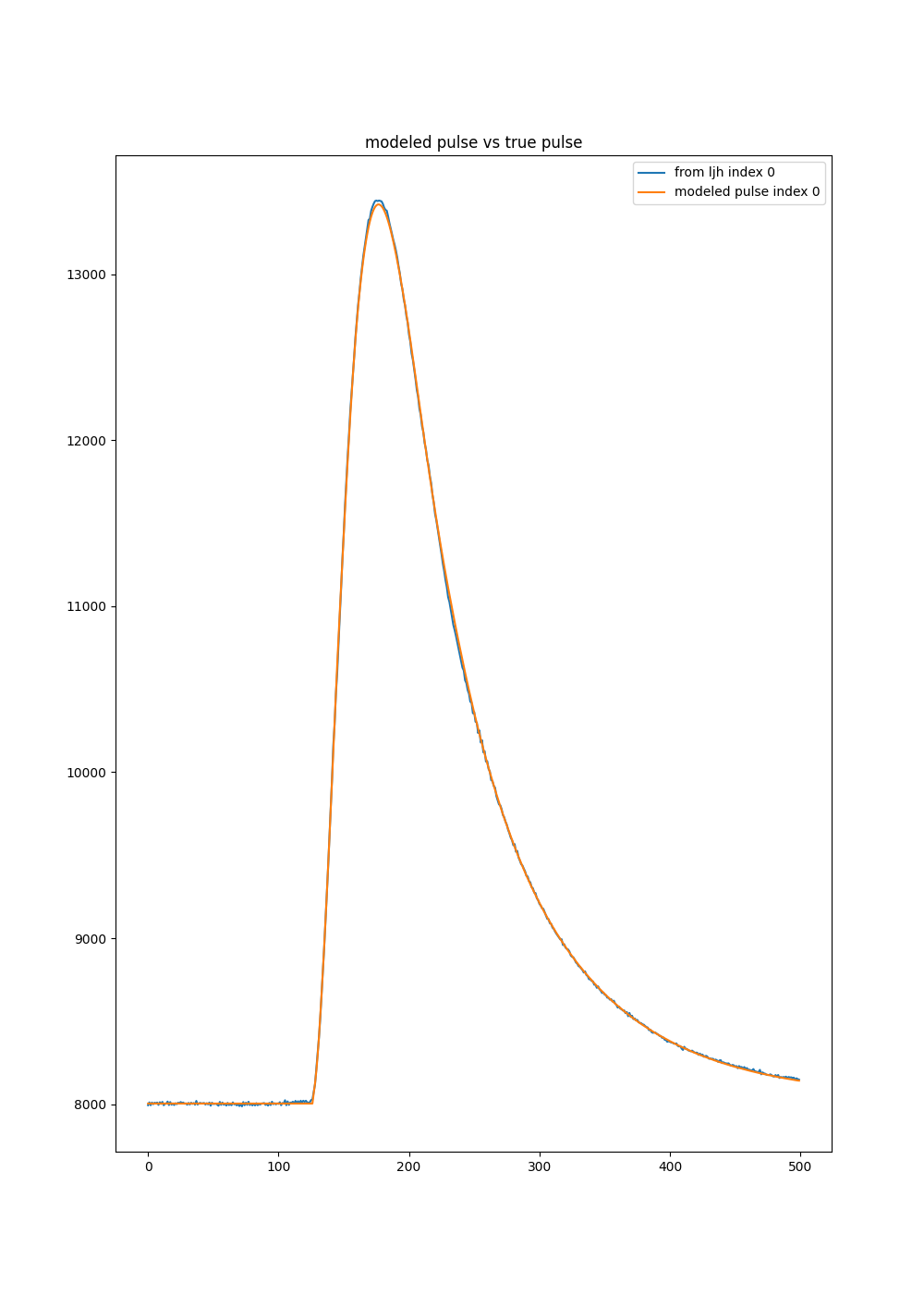
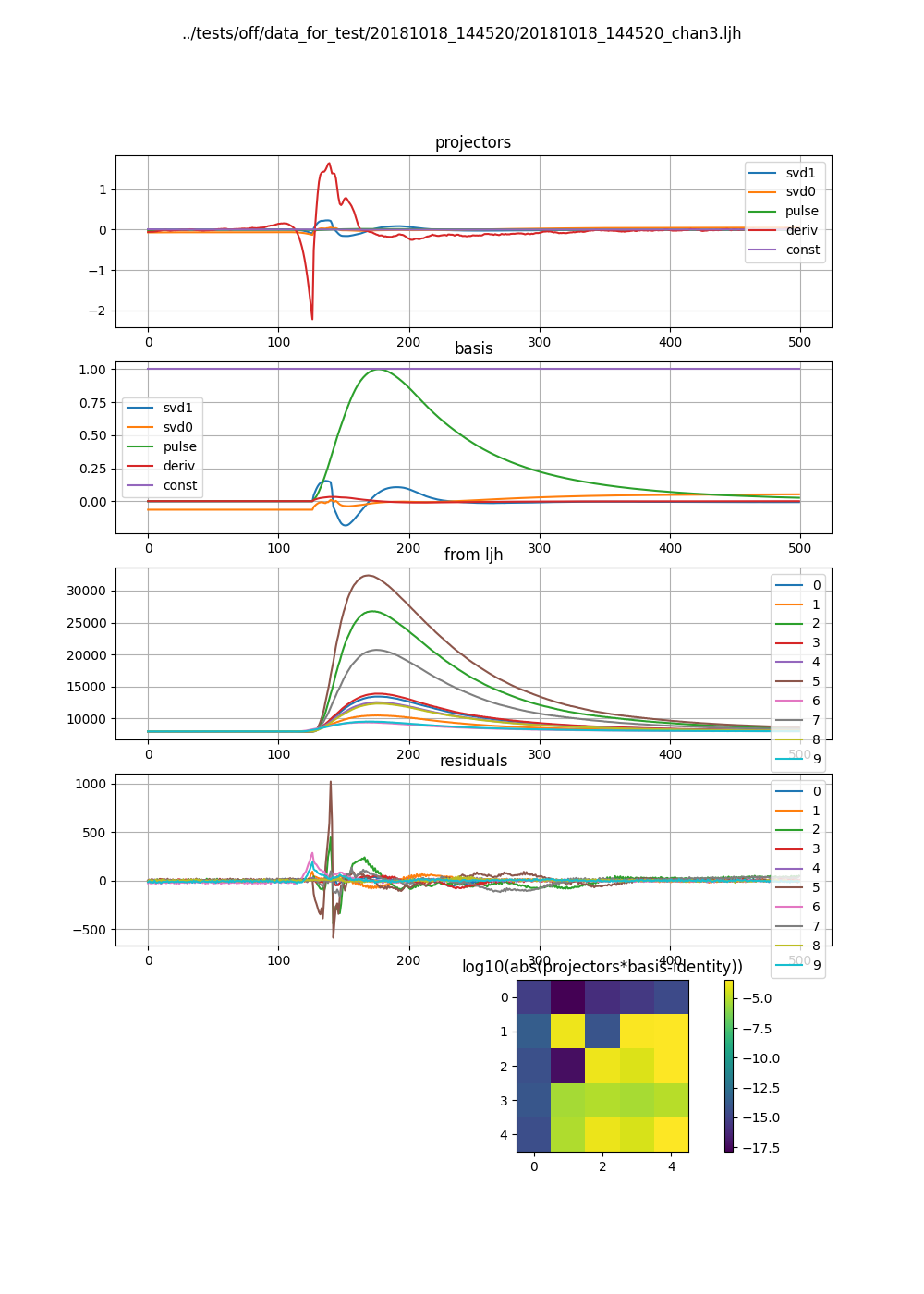
models[3].plot()
Here we plot some info about the “pulse model”, aka the projectors and basis. The right image is larger vertically, so the formatting looks odd.
ljh2off
Then we create off files from the ljh files and the pulse model.
output_dir = os.path.join(d, "20181018_144520_off")
os.mkdir(output_dir)
r = mass.ljh2off.ljh2off_loop(ljhpath = pulse_files[0],
    h5_path = model_hdf5,
    output_dir = output_dir,
    max_channels = 240,
    n_ignore_presamples = 0,
    require_experiment_state=False,
    show_progress=True)
ljh_filenames, off_filenames = r


# write a dummy experiment state file, since the data didn't come with one
with open(os.path.join(output_dir, "20181018_144520_experiment_state.txt"),"w") as f:
    f.write("# yo yo\n")
    f.write("0, START\n")
OFF Analysis
Now we do the off style analysis. The main difference from normal is that we call ds.add5LagRecipes. We need to pass in filter we want to do 5 lags with, and we use the filter generated by made stored in the pulse model file. This requires keeping track fo the pulse model file. It is probably good enough to just truncate the filter stored as the “pulse like” projector in the off file and mean subtract it, but I haven’t dont a careful comparison.
data = ChannelGroup(off_filenames)
data.setDefaultBinsize(10) # set the default bin size in eV for fits

for channum, ds in data.items():
    # define recipes for "filtValue5Lag", "peakX5Lag" and "cba5Lag"
    # where cba refers to the coefficiencts of a polynomial fit to the 5 lags of the filter
    filter_5lag = models[channum].f_5lag
    ds.add5LagRecipes(filter_5lag)
    # this data has artificial offsets of n*2**12 added to pretriggerMean by the phase unwrap algorithm used
    # define a "pretriggerMeanCorrected" to remove these offsets
    ds.recipes.add("pretriggerMeanCorrected", lambda pretriggerMean: pretriggerMean%2**12)
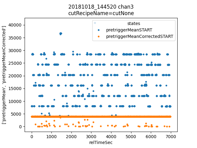
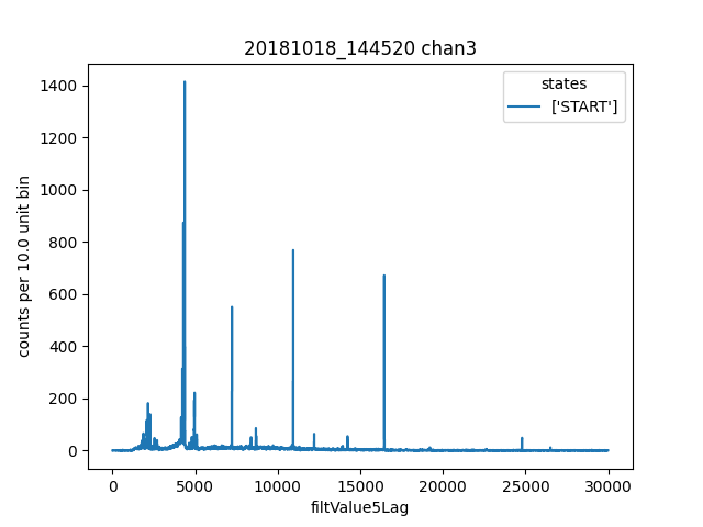
First we check that the pretriggerMeanCorrected value looks better than pretriggerMean. Then we plot a histogram of filtValue5Lag and manually identify lines to add to the calibrationPlan.
ds = data[3]
ds.plotAvsB("relTimeSec", ["pretriggerMean", "pretriggerMeanCorrected"])
ds.plotHist(np.arange(0, 30000, 10),"filtValue5Lag")
ds.calibrationPlanInit("filtValue5Lag")
ds.calibrationPlanAddPoint(4369, 'ErKAlpha1')
ds.calibrationPlanAddPoint(7230, 'Ho166m_80')
ds.calibrationPlanAddPoint(10930, 'Co57_122')
ds.calibrationPlanAddPoint(16450, 'Ho166m_184')
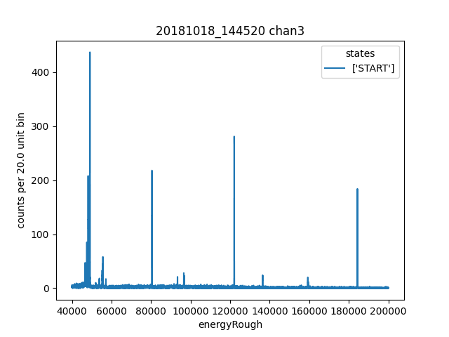
ds.plotHist(np.arange(40000, 200000, 20),"energyRough")
Then we inspect a histogram of energyRough to make sure it seems reasonable.
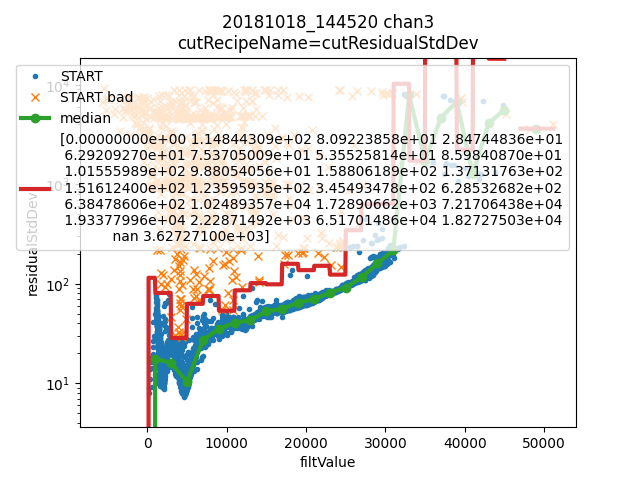
We learn cuts based on residualStdDev, the standard deviation of the residual between the reconstructed pulse and raw pulse data. Then we make a few plots to check for needed corrections and sanity.
# i only want to plot one channel of this
# there is currently no simpler way than this
for ds in data.values()[1:]:
ds.learnResidualStdDevCut(n_sigma_equiv=15, plot=False, setDefault=True)
ds = data[3] # the above loop rebinds ds to the last dataset, but lets keep looking at the same one
ds.learnResidualStdDevCut(n_sigma_equiv=15, plot=True, setDefault=True)
# make a few plots to see if we need corrections
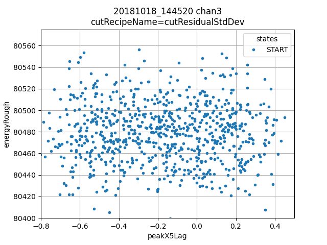
ds.plotAvsB("peakX5Lag", "energyRough")
plt.grid(True)
plt.xlim(-.8, 0.5)
plt.ylim(80400, 80575)
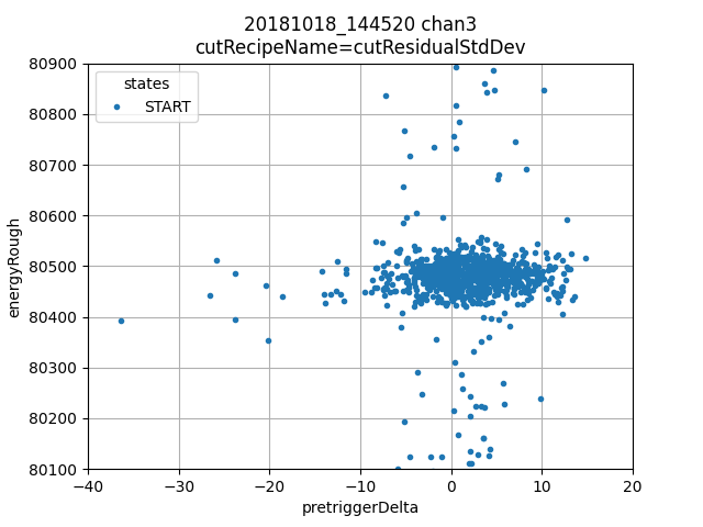
ds.plotAvsB("pretriggerDelta", "energyRough")
plt.grid(True)
plt.xlim(-40, 20)
plt.ylim(80100, 80900)
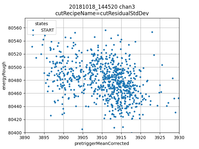
ds.plotAvsB("pretriggerMeanCorrected", "energyRough")
plt.grid(True)
plt.xlim(3890, 3930)
plt.ylim(80400, 80575)
- Various plots:
Top left: the filt value dependent threshold on residualStdDev for a particular channel.
Top right: peakX5lag is an estimator of subsample arrival time, there is possibly some benefit to do further correction, but the 5 lag process has removed the majority of the arrival time effect
Lower left: pretrigger delta is a measure of the slope of the pretrigger region, here we see there are very few pulses with large pretrigger delta and therefore a correction is probably not useful
Lower right: pretriggerMeanCorrection vs energyRough shows a clear slope, in fact it appears to show two slopes or two populations. We will do a correction with a single slope, but it is probably possible to do better, the simplest way would be to cut out the population on the left.
Now we align data, which uses dynamic time warping to identify the peaks in our calibraiton plan in all other channels, creates matching calibration plans for those channels.
We make a special cut for drift correction to only look at energies of interest. We could manually include the cut on residualStdDev by adding it as an argument to the lambda and using another np.logical_and, but I have not done that here. We then learn a drift correction with entropy minimization.
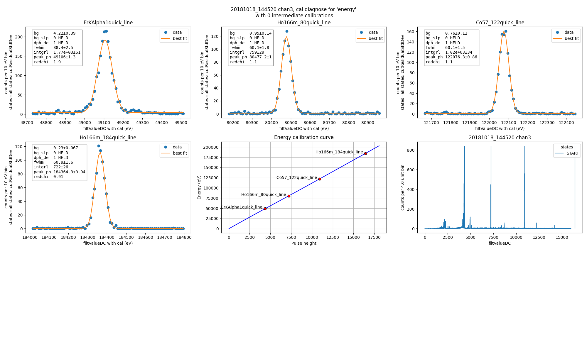
Then we do two seperate calibrations, one with and one without drift correction. Then we call diagnoseCalibration to get a plot of all the fits used for the calibration of one channel.
data.alignToReferenceChannel(ds, "filtValue5Lag", np.arange(0,30000,6))
data.cutAdd("cutEnergyROI", lambda energyRough: np.logical_and(energyRough>40e3,energyRough<200e3), _rethrow=True)
data.learnDriftCorrection(indicatorName="pretriggerMeanCorrected",
    uncorrectedName="filtValue5Lag", correctedName="filtValueDC", cutRecipeName="cutEnergyROI", _rethrow=True)

params = lmfit.Parameters() # use this to adjust params after the guessing routine, eg to hold them fixed
# here the guess routine works well enough so we don't add anything to params
# you can also just leave this out, but I wanted to show that it exists
results_5lag = data.calibrateFollowingPlan("filtValue5Lag", calibratedName="energyNoDC",
    dlo=400, dhi=400,overwriteRecipe=True, params_update = params)
results_dc = data.calibrateFollowingPlan("filtValueDC", calibratedName="energy",
    dlo=400, dhi=400,overwriteRecipe=True, params_update = params)

ds.diagnoseCalibration()
Fit for energy resolution with and without drift correction at the 80 keV line.
# with off style cuts
line = 'Ho166m_80'
for attr in ["energy", "energyNoDC"][:]:
    print(f"{attr}:")
    for ds in data.values():
        result = ds.linefit(line, attr, dlo=200, dhi=200, plot=False, params_update=params)
        if result.params["fwhm"].stderr is None:
            result.params["fwhm"].stderr = 100000
        print(f"""\t{ds.shortName:22} {line} fwhm={result.params["fwhm"].value:.0f} ± {result.params["fwhm"].stderr:.1f}""")
  energy:
      20181018_144520 chan3  Ho166m_80 fwhm=60 ± 1.9
      20181018_144520 chan13 Ho166m_80 fwhm=62 ± 2.0
  energyNoDC:
      20181018_144520 chan3  Ho166m_80 fwhm=64 ± 2.4
      20181018_144520 chan13 Ho166m_80 fwhm=71 ± 2.6
OFF vs Plain Comparision
For many days I thought the Plain mass were about 2 eV better than the OFF style results. I finally tracked the difference down to slighly different ways of fitting the data. Here I do an apples to apples comparison by making sure the histogram bins, cuts, and fitting model and algorithm are all identical between Plain and OFF styles. While off appears slightly better here it is illusory, if you run with different random seeds you can get off to appear worse. Unlike with filtValue, I haven’t been able to get identical results with off vs plain, just comparable. I believe OFF is just as good when you have enough projectors, not better or worse.
We use ds.filtValueDC to access all filtValueDC values without any cuts applied. This may be removed in the future, let me know what you think about it.
# apples to apples comparison to plain mass
for ds in data.values():
plain_ds = data_plain.channel[ds.channum]
e0=mass.STANDARD_FEATURES[line]
bin_edges = np.arange(e0-200, e0+200, 10)
bin_centers = 0.5*(bin_edges[1:]+bin_edges[:-1])
g = plain_ds.good()
cal = plain_ds.calibration["p_filt_value_dc"]
counts, _ = np.histogram(cal(ds.filtValueDC[g]), bin_edges)
model = mass.get_model(line)
params = model.guess(counts, bin_centers, dph_de=1)
params["dph_de"].set(1,vary=False)
result = model.fit(counts, bin_centers=bin_centers, params=params)
fwhm, unc = result.params["fwhm"].value, result.params["fwhm"].stderr
print(f"\tchan {ds.channum:3d} fwhm={fwhm:.1f} ± {unc:.1f} (off)")
plain_counts, _ = np.histogram(cal(plain_ds.p_filt_value_dc[g]), bin_edges)
plain_model = mass.get_model(line)
plain_params = model.guess(plain_counts, bin_centers, dph_de=1)
plain_params["dph_de"].set(1,vary=False)
plain_result = plain_model.fit(plain_counts, bin_centers=bin_centers, params=plain_params)
plain_fwhm, plain_unc = plain_result.params["fwhm"].value, plain_result.params["fwhm"].stderr
print(f"\tchan {ds.channum:3d} fwhm={plain_fwhm:.1f} ± {plain_unc:.1f} (ljh)")
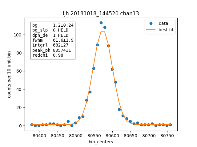
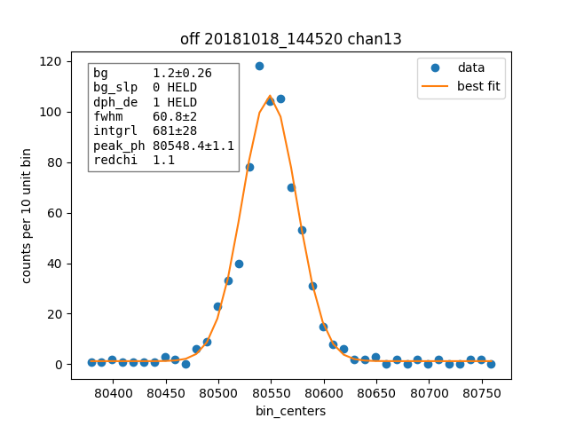
result.plotm(title="off "+ds.shortName)
plain_result.plotm(title="ljh "+ds.shortName)
      chan   3 fwhm=60.0 ± 1.8 (off)
      chan   3 fwhm=60.1 ± 1.8 (ljh)
      chan  13 fwhm=60.8 ± 2.0 (off)
      chan  13 fwhm=61.6 ± 1.9 (ljh)
We also plot one fit from one channel for plain and off style.
Then we compare how many pulses are cut by each cutting approach, remember this would apply to the OFF style resolutions from the previous section, not the apples to apples comparison where we used the same cuts.
# how many were cut
for (ch, ds) in data.items():
    dsp = data_plain.channel[ch]
    print(f"ch {ch}off   ngood={ds.cutResidualStdDev.sum()} ntot={len(ds)}")
    print(f"ch {ch}plain ngood={dsp.good().sum()} ntot={dsp.nPulses}")
  ch 3off   ngood=22112 ntot=22930
  ch 3plain ngood=21715 ntot=22930
  ch 13off   ngood=21498 ntot=22406
  ch 13plain ngood=20423 ntot=22406
Looking into odd pulses
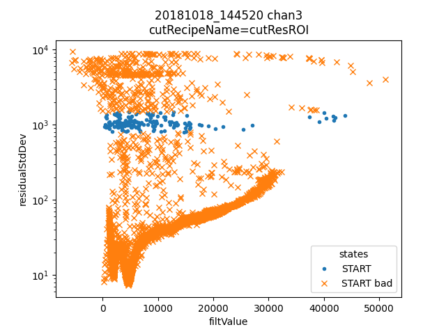
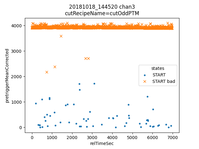
In the residualStdDev plot there is a cluser of pulses with residualStdDev of about 1000 and a second cluster around 5000. Also in the pretriggerMeanCorrected plot there is a large population of pulses with pretriggers of about 0-2000, seperate from the main group at around 4000. Here we will isolate and plot some of those pulses.
ds = data[3]
plain_ds = data_plain.channel[3]
def cutResROI(residualStdDev):
return np.logical_and(residualStdDev>800, residualStdDev<1500)
data.cutAdd("cutResROI", cutResROI)
data.cutAdd("cutOddPTM", lambda pretriggerMeanCorrected: pretriggerMeanCorrected<2000)
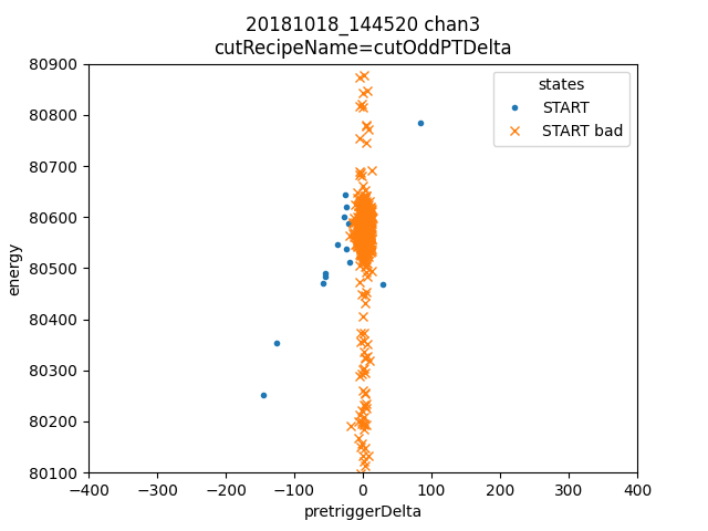
data.cutAdd("cutOddPTDelta", lambda pretriggerDelta, energy: np.logical_and(np.abs(pretriggerDelta)>20,
np.logical_and(energy<80900,
energy>80100)))
ds.plotAvsB("filtValue", "residualStdDev", cutRecipeName="cutResROI", includeBad=True)
plt.yscale("log")
inds = np.nonzero(ds.cutResROI)[0]
plt.figure()
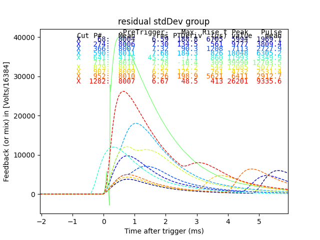
plain_ds.plot_traces(inds[:10], subtract_baseline=True)
plt.title("residual stdDev group")
ds.plotAvsB("relTimeSec","pretriggerMeanCorrected", cutRecipeName="cutOddPTM", includeBad=True)
inds2 = np.nonzero(ds.cutOddPTM)[0]
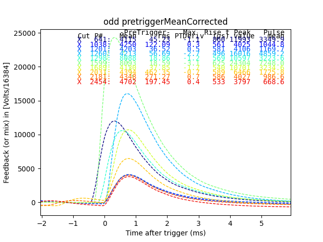
plt.figure()
plain_ds.plot_traces(inds2[:10], subtract_baseline=True)
plt.title("odd pretriggerMeanCorrected")
ds.plotAvsB("pretriggerDelta","energy", cutRecipeName="cutOddPTDelta", includeBad=True)
plt.xlim(-400,400)
plt.ylim(80100, 80900)
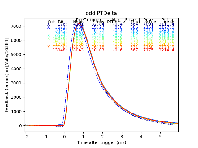
inds3 = np.nonzero(ds.cutOddPTDelta)[0]
plt.figure()
plain_ds.plot_traces(inds3[:10], subtract_baseline=True)
plt.title("odd PTDelta")
Dotted traces were cut by the plain mass analysis. So here we see all the but one of the pulses in the horizontal group of residualStdDev were cut by plain mass. The one that was not cut in plain mass has a phase slip on the rising edge, and should be cut. Many of the others are pulse pile-up events. I suspect that a pulse of constant size causes a roughly constant sized residualStdDev, so the reason there are two bands is that those are the two strongest lines appearing as pileup.
Here we see that many of the odd pretriggerMeanCorrected values come from early triggers, and all were also cut in the plain mass analysis.
Here we look at the pretriggerDelta quantity, designed to replace p_pretrig_rms. I think the pulse records are long enough and the count rates low enough that we don’t see many tails of previous pulses.
Example investigation - Plot energy vs time for good pulses in a narrow window
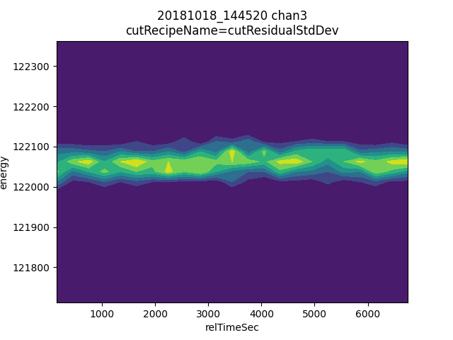
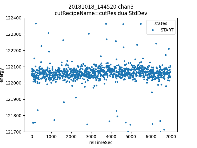
Lets say we want to look at stability of energy vs time, here are some different ways to do that.
ds.plotAvsB("relTimeSec", "energy")
plt.ylim(121.7e3, 122.4e3)
ds.plotAvsB2d("relTimeSec", "energy",  [np.arange(0,7000,300), np.arange(121.7e3,122.4e3,25)])
Warning about defining recipes and closure scope
# this function will be used in the following loop
def f_maker(ch):
    return lambda pretriggerMean: np.zeros(len(pretriggerMean))+ch
for ds in data.values():
    # you may want to define a recipe that depends on some external variable for each ds
    # this is easy to get wrong, so here lets look at the right and wrong way
    ds.recipes.add("channum_wrong", lambda pretriggerMean: np.zeros(len(pretriggerMean))+ds.channum)
    ds.recipes.add("channum_right", f_maker(ds.channum) ) # use a function to introduce new scope, see https://eev.ee/blog/2011/04/24/gotcha-python-scoping-closures/

# you can easily trick yourself that you didnt mess up by writing a loop that defines ds
# this only works because ds happens to have the right value at the time you evaluate the recipe
# but it's really fragile and seems to get "locked in"
for attr in ["channum_wrong", "channum_right"]:
    for ds in data.values():
      v = ds.getAttr(attr, slice(0,1))[0]
      print(f"channel {ds.channum} {attr} gives {v}")
Here the output looks right because ds was changing in the loop.
channel 3 channum_wrong gives 3.0
channel 13 channum_wrong gives 13.0
channel 3 channum_right gives 3.0
channel 13 channum_right gives 13.0
# if we write the loop in a way that doesn't redefine the ds variable, we can see the problem clearly
for attr in ["channum_wrong", "channum_right"]:
    for channum in data.keys():
      v = data[channum].getAttr(attr, slice(0,1))[0]
      print(f"channel {channum} {attr} gives {v}")
Here the output is wrong because we loop in a way that doesnt re-define ds.
channel 3 channum_wrong gives 13.0
channel 13 channum_wrong gives 13.0
channel 3 channum_right gives 3.0
channel 13 channum_right gives 13.0