OFF Style Mass Analysis

Warning

Off style analysis is in development, things will change.

Motivation

OFF files and the associated analysis code and methods were developed to address the following goals:

• High quality spectra available immediatley to provide feedback during experiments

• Faster analysis, for ease of exploratory analysis and to avoid data backlogs

• Improve on the mass design (eg avoid HDF5 file corruption, easier exploratory analysis, simpler code)

• Don’t always start from zero, we generally run the same array on the same spectromter

• Handle experiments with more than one sample (eg calibration sample followed by science sample)

In the previous “mass-style” analysis, as described in Joe Fowler’s “The Practice of Pulse Processing” paper, complete data records are written to disk (LJH files), then analysis starts with generatting optimal filters. In mass-style analysis, new filters are generated for every dataset, and varying experimental conditions (eg sample) are diffuclt to handle, and often handled by writing different files for each condition.

In off-style analysis we start with filters generated exactly the same way, then add more filters that can represent how the pulse shape changes with energy. Data is filtered as it is taken, and only the coefficients of these filter projections are written to disk in OFF files. For now, we typically write both OFF and LJH files just to be safe.

Making Projectors and ljh2off

The script make_projectors will make projectors and write them to disk in a format dastardcommander and ljh2off can use. The script ljh2off can generate off files from ljh files, so you can use this style of analysis on any data, or change your projectors. Call either with a -h flag for help, also all the functionality is available through functions in mass.

Exploring an OFF File

Here we open an OFF file and plot a reconstructed record.

import mass
import numpy as np
import pylab as plt

off = mass.off.OffFile("../tests/off/data_for_test/20181205_BCDEFGHI/20181205_BCDEFGHI_chan1.off")
x,y = off.recordXY(0)

plt.figure()
plt.plot(off.basis[:,::-1]) # put the higher signal to noise components in the front
plt.xlabel("sample number")
plt.ylabel("weight")
plt.legend(["pulseMean","derivativeLike","pulseLike","extra0","extra1"])
plt.title("basis components")

plt.figure()
plt.plot(x,y)
plt.xlabel("time (s)")
plt.ylabel("reconstructed signal (arbs)")
plt.title("example reconstructed pulse")

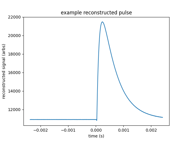
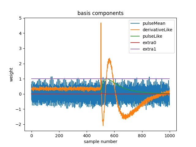
Warning

The basis shown here was generated with obsolete algorithms, and doesn’t look as good as a newer basis will. I should replace it.

What is in a record?

print(off[0])
print(off.dtype)

(1000, 496, 556055239, 1544035816785813000, 10914.036, 22.124851, 10929.741, -10357.827, 10609.358, [-47.434967,  -8.839941])
[('recordSamples', '<i4'), ('recordPreSamples', '<i4'), ('framecount', '<i8'), ('unixnano', '<i8'), ('pretriggerMean', '<f4'), ('residualStdDev', '<f4'), ('pulseMean', '<f4'), ('derivativeLike', '<f4'), ('filtValue', '<f4'), ('extraCoefs', '<f4', (2,))]

recrods of off files numpy arrays with dtypes, which contain may filed. The exact set of fields depends on the off file version as they are still under heavy development. The projector coefficients are stored in “pulseMean”, “derivativeLike”, “filtValue” and “extraCoefs”. You can access

Fields in OFF v3:

• recordSamples - forward looking for when we implement varible length records, the actual number of samples used to calculate the coefficients

• recordPreSamples - forward looking for when we implement varible length records, the actual number of pre-samples used to calculate the coefficients

• framecount - a timestamp in units of DAQ frames (frame = one sample per detector, 0 is related to the start time of DASTARD or the DAQ system)

• unixnano - a timetamp in nanoseconds since the epoch as measured by the computer clock (posix time)

• pretriggerMean - average value of the pre-trigger samples (this may be removed in favor of calculating it from the pulse coefficients)

• residualStdDev - the standard deviation of the residuals of the raw pulse - the reconstructed model pulse

• pulseMean - the mean of the whole pulse record

• derivativeLike - coefficient of the derivativeLike pulse shape

• filtValue - coefficient of the optimal filter pulse shape

• extraCoefs - zero or more additional pulse coefficients one for each other projector used, these generally model pulse shape variation vs energy and are found via SVD

Basic Analysis with a ChannelGroup

Data analysis is generally done within the ChannelGroup class, by convention we call we store it in a variable data and name any particular channel ds. There are convenience functions for many plotting needs, here we plot a histogram of filtValue.

from mass.off import ChannelGroup, getOffFileListFromOneFile, Channel, labelPeak, labelPeaks
data = ChannelGroup(getOffFileListFromOneFile("../tests/off/data_for_test/20181205_BCDEFGHI/20181205_BCDEFGHI_chan1.off", maxChans=2))

I typically just label states alphabetically while taking data, but it can be convenient to alias them with some meaningful name for analysis. Currently this must be done before you access any data from the OFF file.

data.experimentStateFile.aliasState("B", "Ne")
data.experimentStateFile.aliasState("C", "W 1")
data.experimentStateFile.aliasState("D", "Os")
data.experimentStateFile.aliasState("E", "Ar")
data.experimentStateFile.aliasState("F", "Re")
data.experimentStateFile.aliasState("G", "W 2")
data.experimentStateFile.aliasState("H", "CO2")
data.experimentStateFile.aliasState("I", "Ir")

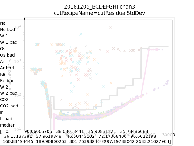
Then we can learn some basic cuts and get an overview of the data.

data.learnResidualStdDevCut(plot=True)
ds = data[1]
ds.plotHist(np.arange(0,25000,10),"filtValue", coAddStates=False)

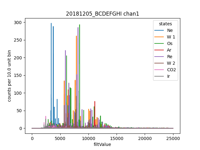
Here we opened all the channels that have the same base filename, plus we opened the _experiment_state.txt that defines states. States provide a convenient way to seperate your data into different chunks by time, and a generally assigned during data aquistion, but you can always make a new _experiment_state.txt file to split things up a different way. This dataset is from an Electron Beam Ion Trap (EBIT) run, and we alias the state names to correspond to the primary element injected into the EBIT during that state. Here W 1 represents the first time Tungsten was injection, since it was injected multiple times.

To calibrate the data we create a CalibrationPlan, for now we do it manually on just one channel. See how we can call out which state or states a paricular line appears in. One a channel has a CalibrationPlan the recipe energyRough will be defined.

from mass.calibration import _highly_charged_ion_lines
data.setDefaultBinsize(0.5)
ds.calibrationPlanInit("filtValue")
ds.calibrationPlanAddPoint(2128, "O He-Like 1s2s+1s2p", states="CO2")
ds.calibrationPlanAddPoint(2421, "O H-Like 2p", states="CO2")
ds.calibrationPlanAddPoint(2864, "O H-Like 3p", states="CO2")
ds.calibrationPlanAddPoint(3404, "Ne He-Like 1s2s+1s2p", states="Ne")
ds.calibrationPlanAddPoint(3768, "Ne H-Like 2p", states="Ne")
ds.calibrationPlanAddPoint(5716, "W Ni-2", states=["W 1", "W 2"])
ds.calibrationPlanAddPoint(6413, "W Ni-4", states=["W 1", "W 2"])
ds.calibrationPlanAddPoint(7641, "W Ni-7", states=["W 1", "W 2"])
ds.calibrationPlanAddPoint(10256, "W Ni-17", states=["W 1", "W 2"])
# ds.calibrationPlanAddPoint(10700, "W Ni-20", states=["W 1", "W 2"])
ds.calibrationPlanAddPoint(11125, "Ar He-Like 1s2s+1s2p", states="Ar")
ds.calibrationPlanAddPoint(11728, "Ar H-Like 2p", states="Ar")

ds.plotHist(np.arange(0, 4000, 1), "energyRough", coAddStates=False)

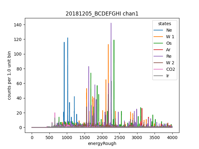
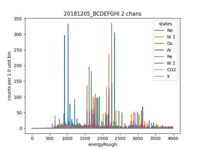
Now we use ds as a reference channel to use dynamitc time warping based alignment to create a matching calibration plan for each other channel. Now we can make co-added energyRough plots. The left plot will be showing how the alignment algorithm works by identifying the same peaks in each channel, and the next will be a coadded energy plot. If alignToReferenceChannel complains, it often helps to increase the range used.

Also notice the coadded plot function is identical to the single channel function, just use it on data. Many function work this way.

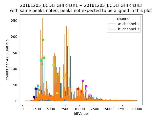
data.alignToReferenceChannel(referenceChannel=ds,
                            binEdges=np.arange(500, 20000, 4), attr="filtValue", _rethrow=True)
aligner = data[3].aligner
aligner.samePeaksPlot()
data.plotHist(np.arange(0, 4000, 1), "energyRough", coAddStates=False)

Now lets learn a correciton to remove some correlation between pretriggerMean and filtValue. First we create a cut recipe to select only pulses in a certain energy range so hopefully the correction will work better in that range. So far, it is not super easy to combine two cuts, but we’ll figure that out eventually, and you can just make a 3rd cut recipe to do so. This will create a recipe for each channel called filtValueDC, though the name can be adjusted with some arguments. There are functions for phase corecction and time drift correction. Don’t expect magic from these, they can only do so much.

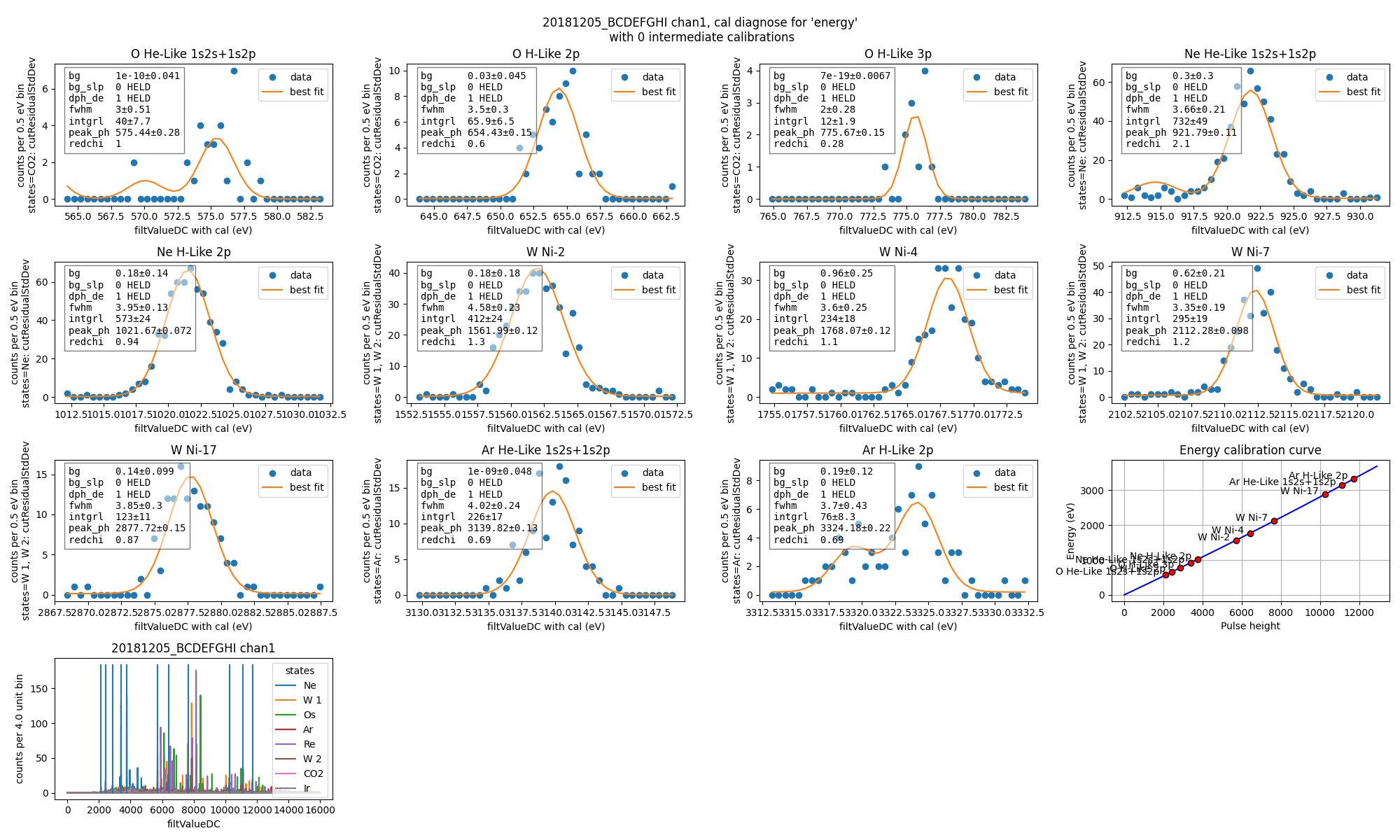
Then we calibrate each channel, using filtValueDC as the input. This creates a recipe energy which is calibrated based on fits to each line in the CalibrationPlan.

data.cutAdd("cutForLearnDC", lambda energyRough: np.logical_and(
    energyRough > 1000, energyRough < 3500), setDefault=False, _rethrow=True)
data.learnDriftCorrection(uncorrectedName="filtValue", indicatorName="pretriggerMean", correctedName="filtValueDC",
  states=["W 1", "W 2"], cutRecipeName="cutForLearnDC", _rethrow=True)
data.calibrateFollowingPlan("filtValueDC", calibratedName="energy", dlo=10, dhi=10, approximate=False, _rethrow=True, overwriteRecipe=True)
ds.diagnoseCalibration()

Then you will often want to fit some lines.

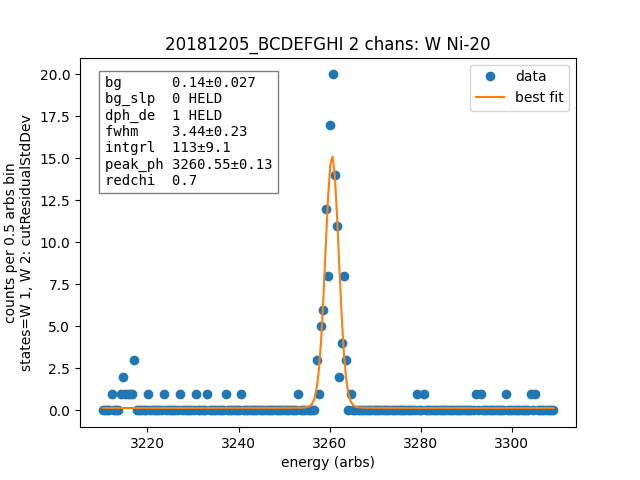
data.linefit("W Ni-20", states=["W 1", "W 2"])

Data

ChannelGroup is a dictionaries of channels. So you may want to loop over them.

for ds in data.values(): # warning this will change the meaning of your existing ds variable
  print(ds)

Channel based on <OFF file> ../tests/off/data_for_test/20181205_BCDEFGHI/20181205_BCDEFGHI_chan1.off, 19445 records, 5 length basis

Channel based on <OFF file> ../tests/off/data_for_test/20181205_BCDEFGHI/20181205_BCDEFGHI_chan3.off, 27369 records, 5 length basis

Bad channels

Some channels will fail various steps of the analysis, or just not be very good. They will be marked bad. I’m also trying to develop some quality check algorithms.

results = data.qualityCheckLinefit("Ne H-Like 3p", positionToleranceAbsolute=2,
                                 worstAllowedFWHM=4.5, states="Ne", _rethrow=True,
                                 resolutionPlot=False)
# all channels here actually pass, so lets pretend they dont
ds.markBad("pretend failure")
print(data.whyChanBad[3])
ds.markGood()

pretend failure

Recipes

During everything in this tutorial, and most off style analsys usage, nothing has been written to disk, and very little is in memory. This is imporant to avoid complicated tracking of state that lead to corruption of HDF5 files in mass, and to allow fast analysis of sub-sets of very large datasets. Most items, eg energy, are computed lazily (on demand) based on a Recipe. Here we can inspect the recipes of ds.

Below I show how to add a recipe and inspect existing recipes.

ds.recipes.add("timeSquared", lambda framecount, relTimeSec: framecount*relTimeSecond)
ds.recipes.add("timePretrig", lambda timeSquared, pretriggerMean: timeSquared*pretriggerMean)
print(ds.recipes)

RecipeBook: baseIngedients=recordSamples, recordPreSamples, framecount, unixnano, pretriggerMean, residualStdDev, pulseMean, derivativeLike, filtValue, extraCoefs, coefs, craftedIngredeints=relTimeSec, filtPhase, cutNone, cutResidualStdDev, energyRough, arbsInRefChannelUnits, cutForLearnDC, filtValueDC, energy, timeSquared, timePretrig

Linefit

X.linefit is a convenience method for quickly fitting a single lines. Here we show some of the options.

import lmfit
# turn off the linear background if you want to later create a composite model, having multiple background functions messes up composite models
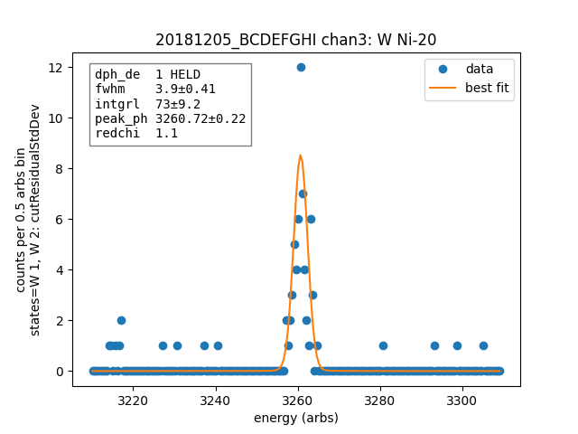
ds.linefit("W Ni-20", states=["W 1", "W 2"], has_linear_background=False)

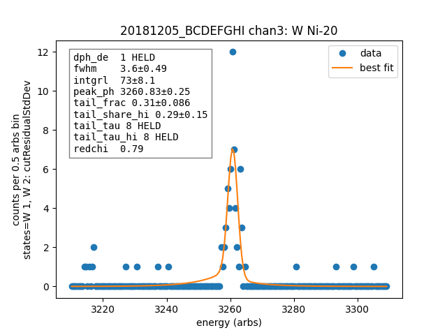
# add tails and specify their parameters
p = lmfit.Parameters()
p.add("tail_frac", value=0.05, min=0, max=1)
p.add("tail_tau", value=8, vary=False)
p.add("tail_share_hi", value=0.20, min=0, max=1)
p.add("tail_tau_hi", value=8, vary=False)
ds.linefit("W Ni-20", states=["W 1", "W 2"], has_linear_background=False, has_tails=True, params_update=p)

Channel

class mass.off.Channel(offFile, experimentStateFile, verbose=True)

Wrap up an OFF file with some convience functions like a TESChannel

add5LagRecipes(f)

alignToReferenceChannel(referenceChannel, attr, binEdges, cutRecipeName=None, _peakLocs=None, states=None)

calibrateFollowingPlan(uncalibratedName, calibratedName='energy', curvetype='gain', approximate=False, dlo=50, dhi=50, binsize=None, plan=None, n_iter=1, method='leastsq_refit', overwriteRecipe=False, has_tails=False, params_update={}, cutRecipeName=None)

calibrationPlanAddPoint(uncalibratedVal, name, states=None, energy=None)

calibrationPlanInit(attr)

cutAdd(cutRecipeName, f, ingredients=None, overwrite=False, setDefault=False)

cutSetDefault(cutRecipeName)

property derivativeLike

diagnoseCalibration(calibratedName='energy', fig=None, filtValuePlotBinEdges=array([0, 4, 8, ..., 15988, 15992, 15996]))

energyTimestampLabelToHDF5(h5File, cutRecipeName=None)

property filtPhase

used as input for phase correction

property filtValue

getAttr(attr, indsOrStates, cutRecipeName=None)

attr - may be a string or a list of strings corresponding to Attrs defined by recipes or the offFile inds - a slice or list of slices returns either a single vector or a list of vectors whose entries correspond to the entries in attr

getStatesIndicies(states=None)

return a list of slices corresponding to the passed states this list is appropriate for passing to _indexOffWithCuts or getRecipeAttr

hist(binEdges, attr, states=None, cutRecipeName=None, calibration=None)

return a tuple of (bin_centers, counts) of p_energy of good pulses (or another attribute). automatically filtes out nan values

binEdges – edges of bins unsed for histogram attr – which attribute to histogram eg “filt_value” cutRecipeName – a function taking a 1d array of vales of type self.offFile.dtype and returning a vector of bool calibration – if not None, transform values by val = calibration(val) before histogramming

histsToHDF5(h5File, binEdges, attr='energy', cutRecipeName=None)

isOffAttr(attr)

isRecipeAttr(attr)

learnChannumAndShortname()

learnDriftCorrection(indicatorName='pretriggerMean', uncorrectedName='filtValue', correctedName=None, states=None, cutRecipeName=None, overwriteRecipe=False)

do a linear correction between the indicator and uncorrected…

learnPhaseCorrection(indicatorName='filtPhase', uncorrectedName='filtValue', correctedName=None, states=None, linePositionsFunc=None, cutRecipeName=None, overwriteRecipe=False)

linePositionsFunc - if None, then use self.calibrationRough._ph as the peak locations otherwise try to call it with self as an argument… Here is an example of how you could use all but one peak from calibrationRough: data.learnPhaseCorrection(linePositionsFunc = lambda ds: ds.recipes[“energyRough”].f._ph

learnResidualStdDevCut(n_sigma_equiv=15, newCutRecipeName='cutResidualStdDev', binSizeFv=2000, minFv=150, states=None, plot=False, setDefault=True, overwriteRecipe=False, cutRecipeName=None)

EXPERIMENTAL: learn a cut based on the residualStdDev. uses the median absolute deviation to estiamte a gaussian sigma that is robust to outliers as a function of filt Value, then uses that to set an upper limit based on n_sigma_equiv highly reccomend that you call it with plot=True on at least a few datasets first

learnTimeDriftCorrection(indicatorName='relTimeSec', uncorrectedName='filtValue', correctedName=None, states=None, cutRecipeName=None, kernel_width=1, sec_per_degree=2000, pulses_per_degree=2000, max_degrees=20, ndeg=None, limit=None, overwriteRecipe=False)

do a polynomial correction based on the indicator you are encouraged to change the settings that affect the degree of the polynomail see help in mass.core.channel.time_drift_correct for details on settings

markBad(reason, extraInfo=None)

markGood()

property nRecords

plotAvsB(nameA, nameB, axis=None, states=None, includeBad=False, cutRecipeName=None)

plotAvsB2d(nameA, nameB, binEdgesAB, axis=None, states=None, cutRecipeName=None, norm=None)

plotCompareDriftCorrect(axis=None, states=None, cutRecipeName=None, includeBad=False)

property pretriggerMean

property pulseMean

qualityCheckDropOneErrors(thresholdAbsolute=None, thresholdSigmaFromMedianAbsoluteValue=None)

qualityCheckLinefit(line, positionToleranceFitSigma=None, worstAllowedFWHM=None, positionToleranceAbsolute=None, attr='energy', states=None, dlo=50, dhi=50, binsize=None, binEdges=None, guessParams=None, cutRecipeName=None, holdvals=None)

calls ds.linefit to fit the given line marks self bad if the fit position is more than toleranceFitSigma*fitSigma away from the correct position

property relTimeSec

property residualStdDev

property rowPeriodSeconds

rowcount

Deprecated since version 0.8.2: Use subframecount, which is equivalent but better named

property statesDict

property subframeDivisions

property subframePeriodSeconds

property subframecount

property unixnano

Channel Group

class mass.off.ChannelGroup(offFileNames, verbose=True, channelClass=<class 'mass.off.channels.Channel'>, experimentStateFile=None, excludeStates='auto')

ChannelGroup is an OrdredDict of Channels with some additional features:

1. Most functions on a Channel can be called on a ChannelGroup, eg data.learnDriftCorrection() in this case it looks over all channels in the ChannelGroup, except those makred bad by ds.markBad(“reason”)

2. If you want to iterate over all Channels, even those marked bad, do

   with data.includeBad:

   for (channum, ds) in data:

   print(channum) # will include bad channels

3. data.whyChanBad returns an OrderedDict of bad channel numbers and reason

calcExternalTriggerTiming(after_last=True, until_next=False, from_nearest=False)

cutSetDefault(cutRecipeName)

firstGoodChannel()

hist(binEdges, attr, states=None, cutRecipeName=None, calibration=None)

return a tuple of (bin_centers, counts) of p_energy of good pulses (or another attribute). Automatically filters out nan values.

binEdges – edges of bins unsed for histogram attr – which attribute to histogram, e.g. “filt_value” calibration – will throw an exception if this is not None

hists(binEdges, attr, states=None, cutRecipeName=None, channums=None)

histsToHDF5(h5File, binEdges, attr='energy', cutRecipeName=None)

Loop over self, calling the histsToHDF5(…) method for each channel. pass _rethrow=True to see stacktrace from first error

histsToHDF5(self, h5File, binEdges, attr=’energy’, cutRecipeName=None) has no docstring

includeBad(x=True)

Use this to do iteration including bad channels temporarily, eg:

with data.includeBad():

for (channum, ds) in data.items():

print(ds)

items() → a set-like object providing a view on D's items

keys() → a set-like object providing a view on D's keys

loadChannels()

loadRecipeBooks(filename)

markAllGood()

outputHDF5Filename(outputDir, addToName='')

plotHists(binEdges, attr, axis=None, labelLines=[], states=None, cutRecipeName=None, maxChans=8, channums=None)

qualityCheckLinefit(line, positionToleranceFitSigma=None, worstAllowedFWHM=None, positionToleranceAbsolute=None, attr='energy', states=None, dlo=50, dhi=50, binsize=None, binEdges=None, guessParams=None, cutRecipeName=None, holdvals=None, resolutionPlot=True, hdf5Group=None, _rethrow=False)

Here we are overwriting the qualityCheckLinefit method created by GroupLooper the call to _qualityCheckLinefit uses the method created by GroupLooper

refreshFromFiles()

refresh from files on disk to reflect new information: longer off files and new experiment states to be called occasionally when running something that updates in real time

resultPlot(lineName, states=None, binsize=None)

saveRecipeBooks(filename)

setDefaultBinsize(binsize)

sets the default binsize in eV used by self.linefit and functions that call it, also sets it for all children

property shortName

values() → an object providing a view on D's values

property whyChanBad