Fitting spectral line models to data in MASS
Designed for MASS version 0.7.3.
Joe Fowler, January 2020.
Previously, we wrote our own modification to the Levenberg-Marquardt optimizer in order to reach maximum-likelihood (not least-squares) fits. This appears in mass as the LineFitter class and its subclasses. In its place, we want to use the LMFIT package and the new MASS class GenericLineModel and its subclasses.
LMFit vs Scipy
LMFIT has numerous advantages over the basic scipy.optimize module. Quoting from the LMFIT documentation, the user can:
forget about the order of variables and refer to Parameters by meaningful names.
place bounds on Parameters as attributes, without worrying about preserving the order of arrays for variables and boundaries.
fix Parameters, without having to rewrite the objective function.
place algebraic constraints on Parameters.
Only some of these are implemented in the original MASS fitters, and even they are not all implemented in the most robust possible way. The one disadvantage of the core LMFIT package is that it minimizes the sum of squares of a vector instead of maximizing the Poisson likelihood. This is easily remedied, however, by replacing the usual computation of residuals with one that computes the square root of the Poisson likelihood contribution from each bin. Voilá! A maximum likelihood fitter for histograms.
Advantages of LMFIT over the earlier, homemade method of the LineFitter include:
Users can forget about the order of variables and refer to Parameters by meaningful names.
Users can place algebraic constraints on Parameters.
The interface for setting upper/lower bounds on parameters and for varying or fixing them is much more elegant, memorable, and simple than our homemade version.
It ultimately wraps the
scipy.optimizepackage and therefore inherits all of its advantages:a choice of over a dozen optimizers with highly technical documentation,
some optimizers that aim for true global (not just local) optimization, and
the countless expert-years that have been invested in perfecting it.
LMFIT automatically computes numerous statistics of each fit including estimated uncertainties, correlations, and multiple quality-of-fit statistics (information criteria as well as chi-square) and offers user-friendly fit reports. See the MinimizerResult object.
It’s the work of Matt Newville, an x-ray scientist responsible for the excellent ifeffit and its successor Larch.
Above all, its documentation is complete, already written, and maintained by not-us.
Usage guide
This overview is hardly complete, but we hope it can be a quick-start guide and also hint at how you can convert your own analysis work from the old to the new, preferred fitting methods.
The underlying spectral line shape models
Objects of the type SpectralLine encode the line shape of a fluorescence line, as a sum of Voigt or Lorentzian distributions. Because they inherit from scipy.stats.rv_continuous, they allow computation of cumulative distribution functions and the simulation of data drawn from the distribution. An example of the creation and usage is:
# In general, known lines are accessed by:
line = mass.spectra["MnKAlpha"]

# But the following is a shortcut for many lines:
line = mass.MnKAlpha

rng = np.random.default_rng(1066)
N = 100000
energies = line.rvs(size=N, instrument_gaussian_fwhm=2.2, rng=rng)  # draw from the distribution
plt.clf()
sim, bin_edges, _ = plt.hist(energies, 120, [5865, 5925], histtype="step");
binsize = bin_edges[1] - bin_edges[0]
e = bin_edges[:-1] + 0.5*binsize
plt.plot(e, line(e, instrument_gaussian_fwhm=2.2)*N*binsize, "k")
plt.xlabel("Energy (eV)")
plt.title("Mn K$\\alpha$ random deviates and theory curve")
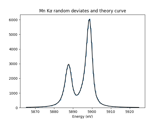
The SpectralLine object is useful to you if you need to generate simulated data, or to plot a line shape, as shown above. Both the new fitting “model” objects and the old “fitter” objects use the SpectralLine object to hold line shape information. You don’t need to create a SpectralLine object for fitting, though; it will be done automatically.
How to use the LMFIT-based models for fitting
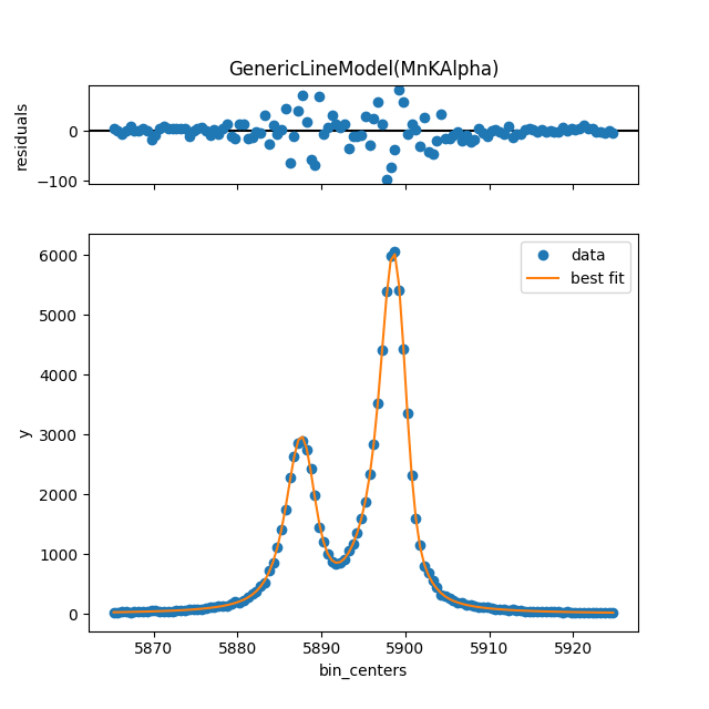
The simplest case of line fitting requires only 3 steps: create a model instance from a SpectralLine, guess its parameters from the data, and perform a fit with this guess. Unlike the old fitters, plotting is not done as part of the fit–you have to do that separately.
model = line.model()
params = model.guess(sim, bin_centers=e, dph_de=1)
resultA = model.fit(sim, params, bin_centers=e)
# Fit again but with dPH/dE held at 1.
# dPH/dE will be a free parameter for the fit by default, largely due to the history of MnKAlpha fits being so critical during development.
# This will not work for nearly monochromatic lines, however, as the resolution (fwhm) and scale (dph_de) are exactly degenerate.
# In practice, most fits are done with dph_de fixed.
params = resultA.params.copy()
resultB = model.fit(sim, params, bin_centers=e, dph_de=1)
params["dph_de"].set(1.0, vary=False)
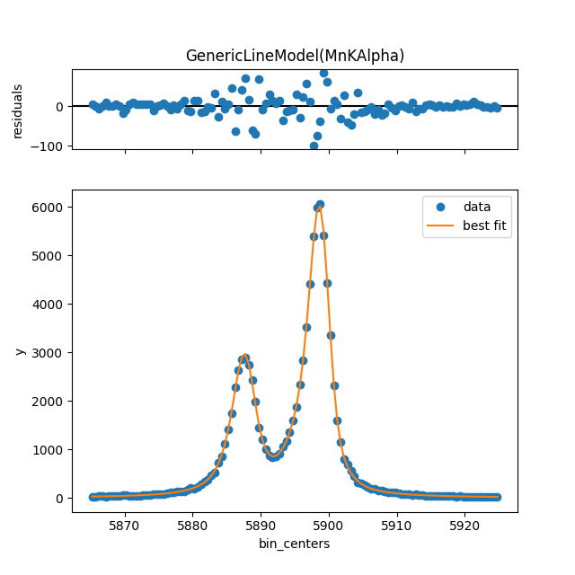
# There are two plotting methods. The first is an LMfit built-in; the other ("mass-style") puts the
# fit parameters on the plot.
resultB.plot()
resultB.plotm()
# The best-fit params are found in resultB.params
# and a dictionary of their values is resultB.best_values.
# The parameters given as an argument to fit are unchanged.
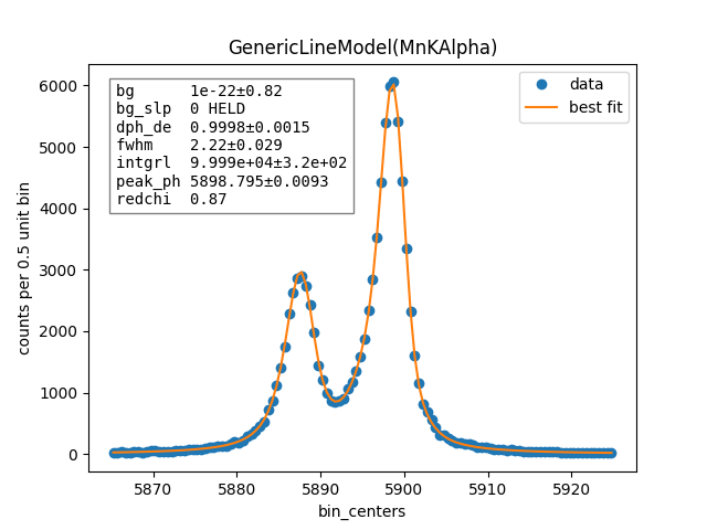
You can print a nicely formatted fit report with fit_report():
print(resultB.fit_report())
[[Model]]
    GenericLineModel(MnKAlpha)
[[Fit Statistics]]
    # fitting method   = least_squares
    # function evals   = 15
    # data points      = 120
    # variables        = 4
    chi-square         = 100.565947
    reduced chi-square = 0.86694782
    Akaike info crit   = -13.2013653
    Bayesian info crit = -2.05139830
    R-squared          = 0.99999953
[[Variables]]
    fwhm:        2.21558094 +/- 0.02687437 (1.21%) (init = 2.217155)
    peak_ph:     5898.79525 +/- 0.00789761 (0.00%) (init = 5898.794)
    dph_de:      1 (fixed)
    integral:    99986.5425 +/- 314.455266 (0.31%) (init = 99985.8)
    background:  5.0098e-16 +/- 0.80578112 (160842446370819488.00%) (init = 2.791565e-09)
    bg_slope:    0 (fixed)
[[Correlations]] (unreported correlations are < 0.100)
    C(integral, background) = -0.3147
    C(fwhm, peak_ph)        = -0.1121
Fitting with exponential tails (to low or high energy)
Notice when you report the fit (or check the contents of the params or resultB.params objects), there are no parameters referring to exponential tails of a Bortels response. That’s because the default fitter assumes a Gaussian response. If you want tails, that’s a constructor argument:
model = line.model(has_tails=True)
params = model.guess(sim, bin_centers=e, dph_de=1)
params["dph_de"].set(1.0, vary=False)
resultC = model.fit(sim, params, bin_centers=e)
resultC.plot()
# print(resultC.fit_report())
By default, the has_tails=True will set up a non-zero low-energy tail and allow it to vary, while the high-energy tail is set to zero amplitude and doesn’t vary. Use these numbered examples if you want to fit for a high-energy tail (1), to fix the low-E tail at some non-zero level (2) or to turn off the low-E tail completely (3):
# 1. To let the low-E and high-E tail both vary simultaneously
params["tail_share_hi"].set(.1, vary=True)
params["tail_tau_hi"].set(30, vary=True)

# 2. To fix the sum of low-E and high-E tail at a 10% level, with low-E tau=30 eV, but
# the share of the low vs high tail can vary
params["tail_frac"].set(.1, vary=False)
params["tail_tau"].set(30, vary=False)

# 3. To turn off low-E tail
params["tail_frac"].set(.1, vary=True)
params["tail_share_hi"].set(1, vary=False)
params["tail_tau"].set(vary=False)
Fitting with a quantum efficiency model
If you want to multiply the line models by a model of the quantum efficiency, you can do that. You need a qemodel function or callable function object that takes an energy (scalar or vector) and returns the corresponding QE. For example, you can use the “Raven1 2019” QE model from mass.materials. The filter-stack models are not terribly fast to run, so it’s best to compute once, spline the results, and pass that spline as the qemodel to line.model(qemodel=qemodel).
raven_filters = mass.materials.efficiency_models.filterstack_models["RAVEN1 2019"]
eknots = np.linspace(100, 20000, 1991)
qevalues = raven_filters(eknots)
qemodel = mass.mathstat.interpolate.CubicSpline(eknots, qevalues)

model = line.model(qemodel=qemodel)
resultD = model.fit(sim, resultB.params, bin_centers=e)
resultD.plotm()
# print(resultD.fit_report())

fit_counts = resultD.params["integral"].value
localqe = qemodel(mass.STANDARD_FEATURES["MnKAlpha"])
fit_observed = fit_counts*localqe
fit_err = resultD.params["integral"].stderr
count_err = fit_err*localqe
print("Fit finds {:.0f}±{:.0f} counts before QE, or {:.0f}±{:.0f} observed. True value {:d}.".format(
    round(fit_counts, -1), round(fit_err, -1), round(fit_observed, -1), round(count_err, -1), N))
Fit finds 168810±530 counts before QE, or 100020±320 observed. True value 100000.

When you fit with a non-trivial QE model, the fit parameters that refer to signal and background intensity all refer to a sensor with an ideal QE=1. These include:
integralbackgroundbg_slope
That is, the fit values must be multiplied by the local QE to give the number of _observed_ signal counts, background counts per bin, or background slope. With or without a QE model, “integral” refers to the number of photons that would be seen across all energies (not just in the range being fit).
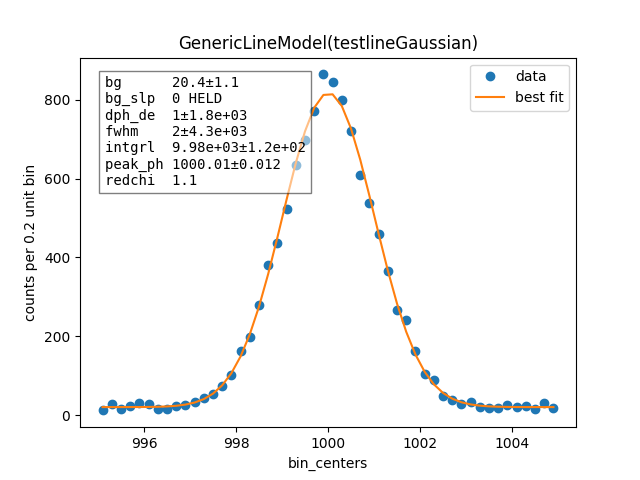
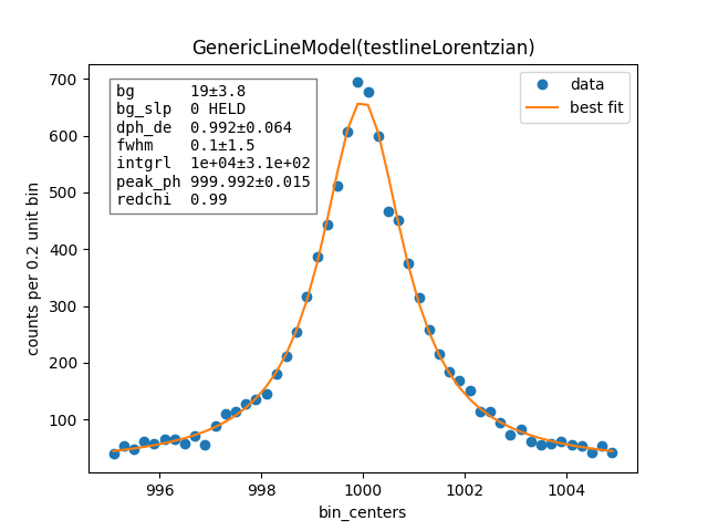
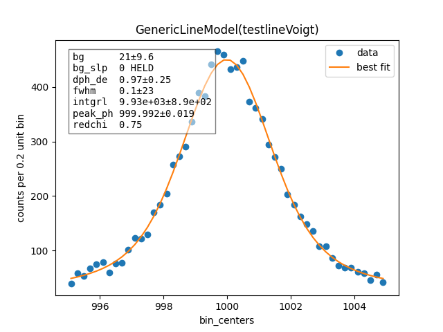
Fitting a simple Gaussian, Lorentzian, or Voigt function
e_ctr = 1000.0
Nsig = 10000
Nbg = 1000

sigma = 1.0
x_gauss = rng.standard_normal(Nsig)*sigma + e_ctr
hwhm = 1.0
x_lorentz = rng.standard_cauchy(Nsig)*hwhm + e_ctr
x_voigt = rng.standard_cauchy(Nsig)*hwhm + rng.standard_normal(Nsig)*sigma + e_ctr
bg = rng.uniform(e_ctr-5, e_ctr+5, size=Nbg)

# Gaussian fit
c, b = np.histogram(np.hstack([x_gauss, bg]), 50, [e_ctr-5, e_ctr+5])
bin_ctr = b[:-1] + (b[1]-b[0]) * 0.5
line = mass.fluorescence_lines.SpectralLine.quick_monochromatic_line("testline", e_ctr, 0, 0)
line.linetype = "Gaussian"
model = line.model()
params = model.guess(c, bin_centers=bin_ctr, dph_de=1)
params["fwhm"].set(2.3548*sigma)
params["background"].set(Nbg/len(c))
resultG = model.fit(c, params, bin_centers=bin_ctr)
resultG.plotm()
# print(resultG.fit_report())

# Lorentzian fit
c, b = np.histogram(np.hstack([x_lorentz, bg]), 50, [e_ctr-5, e_ctr+5])
bin_ctr = b[:-1] + (b[1]-b[0]) * 0.5
line = mass.fluorescence_lines.SpectralLine.quick_monochromatic_line("testline", e_ctr, hwhm*2, 0)
line.linetype = "Lorentzian"
model = line.model()
params = model.guess(c, bin_centers=bin_ctr, dph_de=1)
params["fwhm"].set(2.3548*sigma)
params["background"].set(Nbg/len(c))
resultL = model.fit(c, params, bin_centers=bin_ctr)
resultL.plotm()
# print(resultL.fit_report())

# Voigt fit
c, b = np.histogram(np.hstack([x_voigt, bg]), 50, [e_ctr-5, e_ctr+5])
bin_ctr = b[:-1] + (b[1]-b[0]) * 0.5
line = mass.fluorescence_lines.SpectralLine.quick_monochromatic_line("testline", e_ctr, hwhm*2, sigma)
line.linetype = "Voigt"
model = line.model()
params = model.guess(c, bin_centers=bin_ctr, dph_de=1)
params["fwhm"].set(2.3548*sigma)
params["background"].set(Nbg/len(c))
resultV = model.fit(c, params, bin_centers=bin_ctr)
resultV.plotm()
# print(resultV.fit_report())
How to convert your personal analysis code from the old to the new method
The old “Fitter” methods are very simple to use in the usual case, but they were increasingly klunky if you want to vary what usually doesn’t vary, to hold what usually isn’t held, and to skip plotting, etc. The fitter = mass.MnKAlpha.fitter() is an example of using the old fitters. Don’t do that!
An overview of how to convert is:
Get a Model object instead of a Fitter object.
Use
p=model.guess(data, bin_centers=e, dph_de=dph_de)to create a heuristic for the starting parameters.Change starting values and toggle the
varyattribute on parameters, as needed. For example:p["dph_de"].set(1.0, vary=False)Use
result=model.fit(data, p, bin_centers=e)to perform the fit and store the result.The result holds many attributes and methods (see MinimizerResult for full documentation). These include:
result.params= the model’s best-fit parameters object
result.best_values= a dictionary of the best-fit parameter values
result.best_fit= the model’s y-values at the best-fit parameter values
result.chisqr= the chi-squared statistic of the fit (here, -2log(L))
result.covar= the computed covariance
result.fit_report()= return a pretty-printed string reporting on the fit
result.plot_fit()= make a plot of the data and fit
result.plot_residuals()= make a plot of the residuals (fit-data)
result.plot()= make a plot of the data, fit, and residuals, generally plotm is preferred
result.plotm()= make a plot of the data, fit, and fit params with dataset filename in title
One detail that’s changed: the new models parameterize the tau values (scale lengths of exponential tails) in eV units. The old fitters assumed tau were given in units of bins. Another is that the parameter “integral” refers to the integrated number of counts across all energies; the old parameter “amplitude” was the same but scaled by the bin width in eV. The old way didn’t make sense, but that’s how it was.
To do
[x] We probably should restructure the
SpectralLine,GenericLineModel, and perhaps also the olderLineFitterobjects such that the specific versions for (say) Mn Kα become not subclasses but instances of them. See issue 182 on the question of whether this change might speed up loading of MASS. Done by PR#120.[x] Add to
GenericLineModelone or more methods to make plots comparing data and fit with parameter values printed on the plot.[x] The LMFIT view of models is such that we would probably find it easy to fit one histogram for the sum of (say) a Mn Kα and a Cr Kβ line simultaneously. Add features to our object, as needed, and document the procedure here.
[ ] We could implement convolution between two models (see just below CompositeModel in the docs for how to do this).
[x] At some point, we ought to remove the deprecated
LineFitterobject and subclasses thereof.