Detector X-ray Efficiency Models
Warning
This module requires the xraydb python package. You should be able to install with ‘sudo pip install xraydb’.
Motivation
For many analyses, it is important to estimate a x-ray spectrum as it would be seen from the source rather than as it would be measured with a set of detectors. This can be important, for example, when trying to determine line intensity ratios of two lines separated in energy space. Here, we attempt to model the effects that would cause the measured spectrum to be different from the true spectrum, such as energy dependent losses in transmission due to IR blocking filters and vacuum windows. Energy dependent absorber efficiency can also be modeled.
FilterStack class and subclass functions with premade efficiency models
Here, we import the mass.efficiency_models module and demonstrate the functionality with some of the premade efficiency models.
Generally, these premade models are put in place for TES instruments with well known absorber and filter stack compositions.
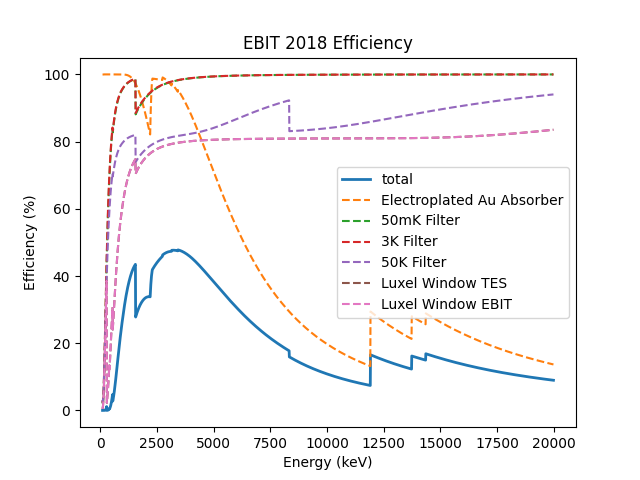
To demonstrate, we work with the ‘EBIT 2018’ model, which models the TES spectrometer setup at the NIST EBIT, as it was commissioned in 2018.
This model includes a ~1um thick absorber, 3 ~100nm thick Al IR blocking filters, and LEX HT vacuum windows for both the TES and EBIT vacuums.
We begin by importing efficiency_models and examining the EBIT efficiency model components.
We can see that the model is made of many submodels (aka components) and that all the parameters have uncertainties. The EBIT system was particularly well characterized, so the uncertainties are fairly low. The presence of uncertainties requires some special handling in a few places, these docs will show some examples.
import mass
import mass.materials  # you have to explicitly import mass.materials
import numpy as np
import pylab as plt
from uncertainties import unumpy as unp  # useful for working with arrays with uncertainties aka uarray
from uncertainties import ufloat

EBIT_model = mass.materials.filterstack_models['EBIT 2018']
print(EBIT_model)
<class 'mass.materials.efficiency_models.FilterStack'>(
Electroplated Au Absorber: <class 'mass.materials.efficiency_models.Film'>(Au 0.00186+/-0.00006 g/cm^2, fill_fraction=1.000+/-0, absorber=True)
50mK Filter: <class 'mass.materials.efficiency_models.AlFilmWithOxide'>(Al (3.04+/-0.06)e-05 g/cm^2, Al 1.27e-06 g/cm^2, O 1.13e-06 g/cm^2, fill_fraction=1.000+/-1.000, absorber=False)
3K Filter: <class 'mass.materials.efficiency_models.AlFilmWithOxide'>(Al (2.93+/-0.06)e-05 g/cm^2, Al 1.27e-06 g/cm^2, O 1.13e-06 g/cm^2, fill_fraction=1.000+/-1.000, absorber=False)
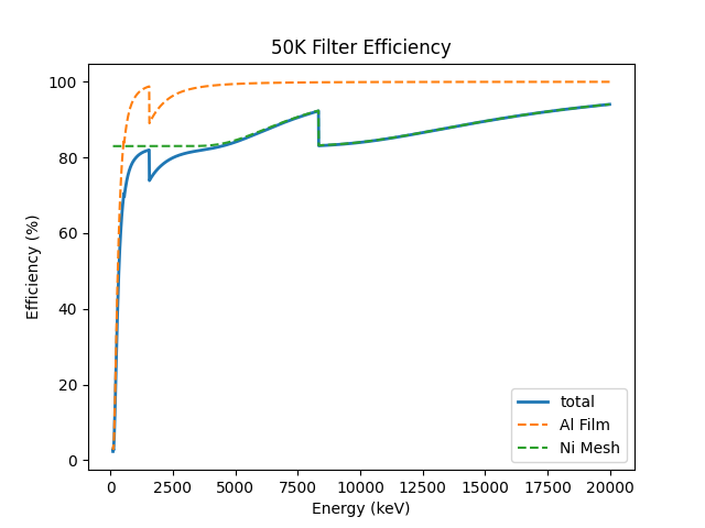
50K Filter: <class 'mass.materials.efficiency_models.FilterStack'>(
Al Film: <class 'mass.materials.efficiency_models.AlFilmWithOxide'>(Al (2.77+/-0.06)e-05 g/cm^2, Al 1.27e-06 g/cm^2, O 1.13e-06 g/cm^2, fill_fraction=1.000+/-1.000, absorber=False)
Ni Mesh: <class 'mass.materials.efficiency_models.Film'>(Ni 0.0134+/-0.0018 g/cm^2, fill_fraction=0.170+/-0.010, absorber=False)
)
Luxel Window TES: <class 'mass.materials.efficiency_models.LEX_HT'>(
LEX_HT Film: <class 'mass.materials.efficiency_models.Film'>(C (6.70+/-0.20)e-05 g/cm^2, H (2.60+/-0.08)e-06 g/cm^2, N (7.20+/-0.22)e-06 g/cm^2, O (1.70+/-0.05)e-05 g/cm^2, Al (1.70+/-0.05)e-05 g/cm^2, fill_fraction=1.000+/-0, absorber=False)
LEX_HT Mesh: <class 'mass.materials.efficiency_models.Film'>(Fe 0.0564+/-0.0011 g/cm^2, Cr 0.0152+/-0.0003 g/cm^2, Ni 0.00720+/-0.00014 g/cm^2, Mn 0.000800+/-0.000016 g/cm^2, Si 0.000400+/-0.000008 g/cm^2, fill_fraction=0.190+/-0.010, absorber=False)
)
Luxel Window EBIT: <class 'mass.materials.efficiency_models.LEX_HT'>(
LEX_HT Film: <class 'mass.materials.efficiency_models.Film'>(C (6.70+/-0.20)e-05 g/cm^2, H (2.60+/-0.08)e-06 g/cm^2, N (7.20+/-0.22)e-06 g/cm^2, O (1.70+/-0.05)e-05 g/cm^2, Al (1.70+/-0.05)e-05 g/cm^2, fill_fraction=1.000+/-0, absorber=False)
LEX_HT Mesh: <class 'mass.materials.efficiency_models.Film'>(Fe 0.0564+/-0.0011 g/cm^2, Cr 0.0152+/-0.0003 g/cm^2, Ni 0.00720+/-0.00014 g/cm^2, Mn 0.000800+/-0.000016 g/cm^2, Si 0.000400+/-0.000008 g/cm^2, fill_fraction=0.190+/-0.010, absorber=False)
)
)
Next, we examine the function get_efficiency(xray_energies_eV), which is an attribute of FilterStack.
This can be called for the entire filter stack or for individual components in the filter stack.
As an example, we look at the efficiency of the EBIT 2018 filter stack and the 50K filter component between
2,000 eV and 10,000 eV, at 1,000 eV steps.
sparse_xray_energies_eV = np.arange(2000, 10000, 1000)
stack_efficiency = EBIT_model.get_efficiency(sparse_xray_energies_eV)
stack_efficiency_uncertain = EBIT_model.get_efficiency(sparse_xray_energies_eV, uncertain=True) # you have to opt into getting uncertainties out
filter50K_efficiency = EBIT_model.components['50K Filter'].get_efficiency(sparse_xray_energies_eV)

print("stack efficiencies")
print([f"{x}" for x in stack_efficiency_uncertain]) # this is a hack to get uarrays to print with auto chosen number of sig figs
print(stack_efficiency) # this is a hack to get uarrays to print with auto chosen number of sig figs
print(unp.nominal_values(stack_efficiency)) # you can easily strip uncertainties, see uncertains package docs for more info

print("filter50K efficiencies")
print(filter50K_efficiency) # if you want to remove the uncertainties, eg for plotting
stack efficiencies
['0.34+/-0.04', '0.472+/-0.022', '0.456+/-0.014', '0.383+/-0.011', '0.307+/-0.009', '0.242+/-0.008', '0.191+/-0.006', '0.136+/-0.005']
[0.33535662 0.4719283  0.45559501 0.38309458 0.30687859 0.24201976
 0.19141294 0.13581482]
[0.33535662 0.4719283  0.45559501 0.38309458 0.30687859 0.24201976
 0.19141294 0.13581482]
filter50K efficiencies
[0.77672107 0.81107679 0.8233861  0.84072724 0.86670307 0.89357999
 0.9163624  0.83360284]
Here, we use the function plot_efficiency(xray_energies_eV, ax) to plot the efficiencies.
ax defaults to None, but can be used to plot the efficiencies on a user provided axis.
Just like get_efficiency, plot_efficiency works with FilterStack and its subclasses.
Testing with energy range 100 to 20,000 eV, 1 eV steps.
xray_energies_eV = np.arange(100,20000,10)
EBIT_model.plot_efficiency(xray_energies_eV)
EBIT_model.components['50K Filter'].plot_efficiency(xray_energies_eV)
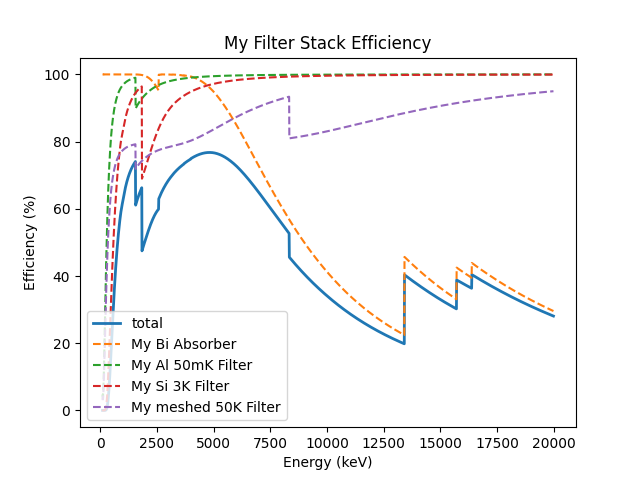
Creating your own custom filter stack model using FilterStack objects
Now we will explore creating custom FilterStack objects and building up your very own filter stack model.
First, we will create a general FilterStack object, representing a stack of filters.
We will then populate this object with filters, which take the form of the various FilterStack object subclasses, such as Film,
or even other FilterStack objects to create more complicated filters with multiple components.
The add argument can be used to add a premade FilterStack object as a component of a different FilterStack object.
We will start by adding some simple Film objects to the filter stack.
This class requires a the name and material arguments, and the optical depth can be specified by passing in either
area_density_g_per_cm2 or thickness_nm (but not both).
By default, most FilterStack objects use the bulk density of a material to calculate the optical depth when the thickness_nm is used,
but a custom density can be specified with the density_g_per_cm3 argument.
In addition, a meshed style filter can be modelled using the fill_fraction argument.
Finally, most FilterStack subclasses can use the absorber argument (default False), which will cause the object to return absorption,
instead of transmittance, as the efficiency.
All numerical arguments can be passed with our without uncertainties. If you don’t have at least one number with specified uncertainty in a particular Film, the code will add a +/- 100% uncertainty on that component. This way, hopefully you will notice that your uncertainty is higher than you expect, and double check the inputs. Read up on the uncertainties package for more info about how it works.
custom_model = mass.materials.FilterStack(name='My Filter Stack')
custom_model.add_Film(name='My Bi Absorber', material='Bi', thickness_nm=ufloat(4.0e3, .1e3), absorber=True)
custom_model.add_Film(name='My Al 50mK Filter', material='Al', thickness_nm=ufloat(100.0, 10))
custom_model.add_Film(name='My Si 3K Filter', material='Si', thickness_nm=ufloat(500.0, 2))
custom_filter = mass.materials.FilterStack(name='My meshed 50K Filter')
custom_filter.add_Film(name='Al Film', material='Al', thickness_nm=ufloat(100.0, 10))
custom_filter.add_Film(name='Ni Mesh', material='Ni', thickness_nm=ufloat(10.0e3, .1e3), fill_fraction=ufloat(0.2, 0.01))
custom_model.add(custom_filter)

custom_model.plot_efficiency(xray_energies_eV)
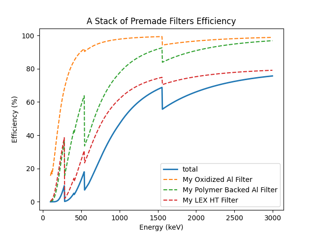
There are also some premade filter classes for filters that commonly show up in our instrument filter stacks.
At the moment, the FilterStack subclasses listed below are implemented:
- AlFilmWithOxide - models a typical IR blocking filter with native oxide layers, which can be important for thin filters.
- AlFilmWithPolymer - models a similar IR blocking filter, but with increased structural support from a polymer backing.
- LEX_HT - models LEX_HT vacuum windows, which contain a polymer backed Al film and stainless steel mesh.
Usage examples and efficiency curves of these classes are shown below.
premade_filter_stack = mass.materials.FilterStack(name='A Stack of Premade Filters')
premade_filter_stack.add_AlFilmWithOxide(name='My Oxidized Al Filter', Al_thickness_nm=50.0)
premade_filter_stack.add_AlFilmWithPolymer(name='My Polymer Backed Al Filter', Al_thickness_nm=100.0, polymer_thickness_nm=200.0)
premade_filter_stack.add_LEX_HT(name='My LEX HT Filter')
low_xray_energies_eV = np.arange(100,3000,5)
premade_filter_stack.plot_efficiency(low_xray_energies_eV)